With American election season in full swing, at least as I write this (February 1st, 2024), I thought it might be appropriate to write about Benford’s law, how it has been used in the past to analyze numbers, why it has been used to search for election fraud, and, importantly, when it is inappropriate to apply Benford’s law.
Numbers, in nature, will often follow patterns, and one particular pattern pops up in so many disparate data sets that some are comfortable throwing up their hands and claiming it to be magic. I speak of course of the famous Law of Anomalous Numbers.
In certain data sets, there is a pattern in the frequency of the leading digit, this was noticed by Simon Newcomb who first observed it in 18811. As a physicist, he was often looking up numbers in log tables and made a curious observation: the earlier pages in the book of log tables were more tattered than the later pages. He wondered if this was a pattern repeated elsewhere. Benford expounded upon his work and wrote a paper in 1938 titled “The Law of Anomalous Numbers” and this phenomenon is now called Benford’s law, the Newcomb-Benford law, or the Law of Anomalous Numbers. This pattern can be found in quite a wide variety of natural phenomenon, sometimes it is intuitive as to why the pattern emerges, sometimes not; and it will emerge in some rather strange places at times.
Definition
Benford’s law concerns itself with only the leading digits in a list of numbers. The leading digit is simply the number in the front. So, for example, the number 3,427,846 has a leading digit of 3. We are not at all interested in any other digits in the number except for the lead digit.
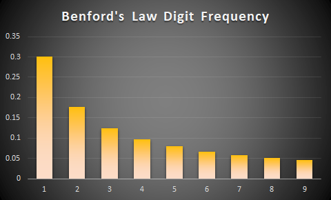
In a given dataset, according to Benford’s law, about 30% of the leading digits will be 1, about 17% will be 2, 12% will be 3, and the frequency of the digits decreases as they get larger. The specific calculation is for frequency is:
![\[\log_{10}(n+1) - \log_{10} (n) \]](https://lejavbasolutions.com/wp-content/ql-cache/quicklatex.com-4f993aec1c4ce6eb454e37953a8640f1_l3.png "Rendered by QuickLaTeX.com")
And when graphed looks like so:
That pattern’s origins are easier to see when looking at a log scale:
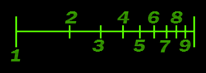
Start marking random locations on the above line, there is a roughly 30% chance it will be 1, a 17% chance it will be 2, etc.
The law in nature:
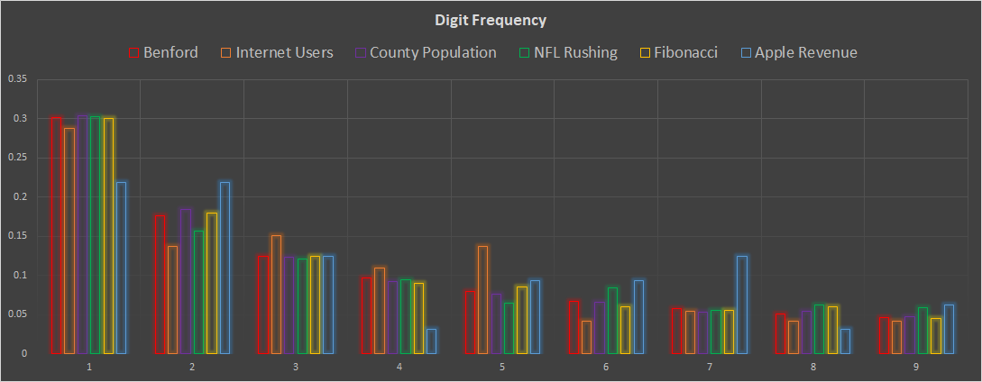
I have gathered some data from seemingly unrelated fields and graphed them. All of these pass the tests (introduced below) and exhibit a Benford pattern: The number of internet users over time2, the population figures for US counties, the number of rushing yards by player for the 2023 NFL season3, the Fibonacci sequence of numbers, and Apple’s revenue since 19924.
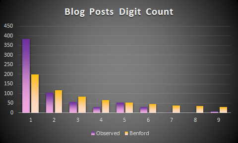
Mixed numbers, surprisingly, often conform. A mixed number might be taking all numbers from a body of text. Benford himself did this using Reader’s Digest. He went through the text, took all the numbers out and isolated the first digits. This set, too, conformed. I performed the same trick with my own blog posts, however, I do not get conformity. Perhaps my dataset is too small and over time, it will conform (I write slowly).
The following is a list of distributions tested by Benford:
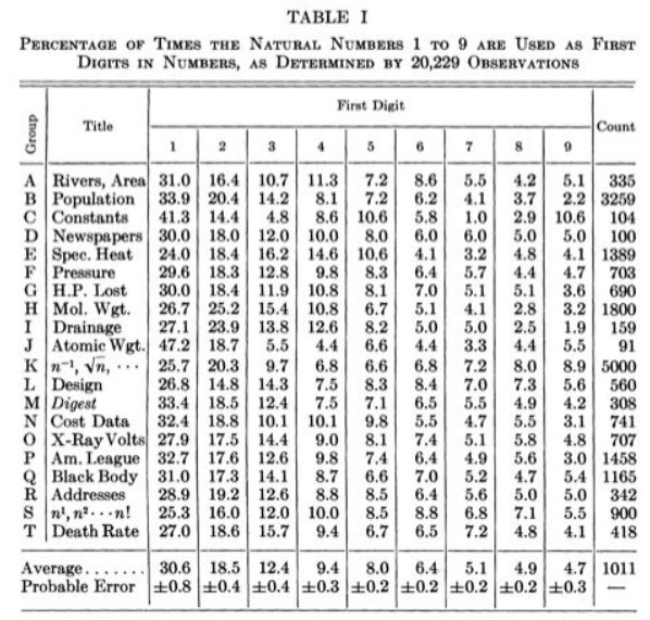
The pervasiveness of the law is quite clear. And it is more than a mere parlor trick. This is a real phenomenon in statistics that has really been used to discover fraudulent data from accounting to elections and is admissible in court6. This paper utilized Benford’s law to test whether an image is real or computer generated. The analytical power cannot be denied. However, and this is extremely important, it must be applied correctly to appropriate data sets and even then, any violations must be treated as a red flag at best!
Commonalities and expectations and deviations:
Datasets which conform generally share some similarities. They tend to be larger data sets, so  is large. The data ranges over orders of magnitude. Not just 1-9 but maybe 1- 100,000 or even in the millions or billions. Exponential growth models conform very well, as shown below.
Data sets where it is less likely to find conformity include sets of assigned numbers. For example zip codes, precinct sizes, and area codes. Sets with upper and lower bounds, set either naturally or arbitrarily, will likely not conform either; examples include rolling a die (the maximum number is capped at 6) or human weight (very few humans weigh less than 20 kg).
When humans falsify data, they often do so poorly, or just sloppily. Take, for example, the recent case of disgraced politician George Santos7. According to the congressional reporting standards, any political spending greater than $200 must be reported. When analysists became suspicious about the number of Santos’s finances, they found a vast number of purchases for exactly $199.99. This type of forgery is simply lazy, but works to highlight another point. Imagine a nefarious person is attempting to falsify numbers. Maybe they want to be more sophisticated than Santos, so they employ a random number generator. What could be more natural than random? Well, as shown, numbers may have hidden distributions and patterns, so when an expected pattern doesn’t emerge, that opens the door for statisticians and analysts to start asking questions. To illustrate, first I want to compare random numbers to the Benford distribution. Then I will create a dataset that conforms quite nicely before finally testing some election vote totals.

I would like to make a column of random numbers ranging from 1 to 9,999,999 to see if any pattern emerges. To do so, simply use the randombetween function and drag it down to however many rows you’d like. I chose 10,000 rows.
=RANDBETWEEN(1,9999999)
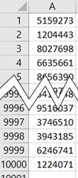
And isolate the first digit of each of those numbers:
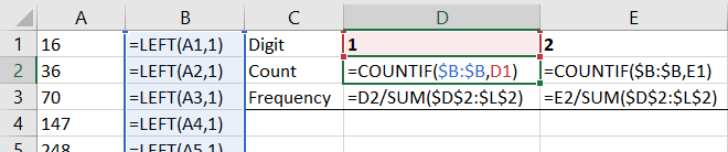
In Excel, this is easily achieved using the LEFT formula =LEFT(cell, desired number of characters). This formula returns only the desired number of characters in the cell, starting from the left.
(The RIGHT formula does that exact same thing, only counting from the rightmost character.)
Next, count them up, how many are 1’s, how many are 2’s etc. in order to see how often each number shows up. This is also called frequency, how frequent is each number?
I achieved this using the COUNTIF formula. =COUNTIF(range, value) By changing value to 1, this formula will count all the number of cells that hold “1”. By changing value to 2, this formula will count all the number of cells that hold “2”, etc.
To get the frequency of each digit, simply divide the count by the total number of observations.
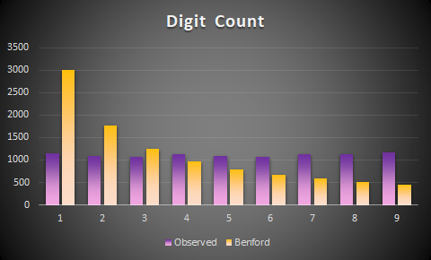
Graphing them together, it is clear that there is no conformity between the law and the list of random numbers.
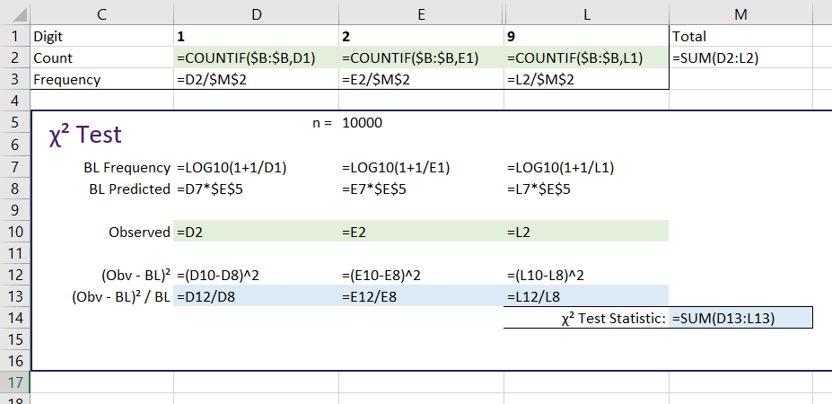
Nonetheless, I would like to also use two, more rigorous, statistical tests to check for conformity. The first one is the Chi-squared test. This test is fairly simple and requires only two components: the expected frequency of numbers via  , and the actual frequency given by the Excel COUNTIF functions. In other words, the expected values and the actual or observed values. I use the chi-squared in conjunction with another test to paint a fuller picture.
To perform the chi-squared, simply take the expected value, subtract off the actual value, square that number, then divide it by the expected value.
![\[\frac{(Obs_1 - Expected_1)^2}{Expected_1}\]](https://lejavbasolutions.com/wp-content/ql-cache/quicklatex.com-50e6d9d96ac51aaa0cc099b17878d401_l3.png "Rendered by QuickLaTeX.com")
Do that nine times, for each integer 1 to 9 and add them.
![\[\frac{(Obs_1 - Expected_1)^2}{Expected_1} + \frac{(Obs_2 - Expected_2)^2}{Expected_2} \dotsi \frac{(Obs_9 - Expected_9)^2}{Expected_9}\]](https://lejavbasolutions.com/wp-content/ql-cache/quicklatex.com-babaaf299a0d06cd90acfe3c00c2d40d_l3.png "Rendered by QuickLaTeX.com")
Sum the above
![\[ \sum_{i=1}^{9} \frac{(Obs_i - Expected_i)^2}{Expected_i}\]](https://lejavbasolutions.com/wp-content/ql-cache/quicklatex.com-aac5ae5376a3bc0d8b18fa97c2b1ddd5_l3.png "Rendered by QuickLaTeX.com")
This results in the test value, we can compare that to the critical value, calculated beforehand in the chi-squared table. There are n-1 degrees of freedom, n is 9, so we want to look up the chi-squared critical value with 8 degrees of freedom. By convention, a 95% confidence level is chosen. I have added the confidence levels of 90%, 95%, 97.5%, 99%, and 99.9%.
For the chi-squared test, the null hypothesis is that the data conforms to the expected distribution. The alternative hypothesis is that it does not.
 : The observed data follows a Benford’s law distribution.
 : The observed data does not follow a Benford’s law distribution.
If the test value is greater than, or more extreme than, the critical value, we reject and conclude that the data does not conform to Benford’s law. Here are the formulas ( some columns hidden):
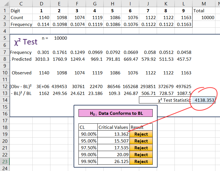
Test Statistic > Critical Value therefore reject
It is quite clear that, with a test statistic of greater than 4,138, the null hypothesis is rejected at all levels: the random list of 10,000 numbers does not follow a Benford’s law distribution in any way.
Turning to the second test, this one is called the Cho & Gaines’s Distance test and uses the following formula:
![\[d = \sqrt{N \times \sum_{i=1}^{9}\left[ (Pr(X = i) - \log_{10}\left(1+\frac{1}{i}\right)\right]^2\]](https://lejavbasolutions.com/wp-content/ql-cache/quicklatex.com-160814b54b8a0ea835ae7b81b7bf10d4_l3.png "Rendered by QuickLaTeX.com")
This test looks similar to the chi-squared test but is instead calculated using the frequency of the numbers instead of the count of the numbers. More can be read about this test and it’s critical values here8.
The results of the distance test are:
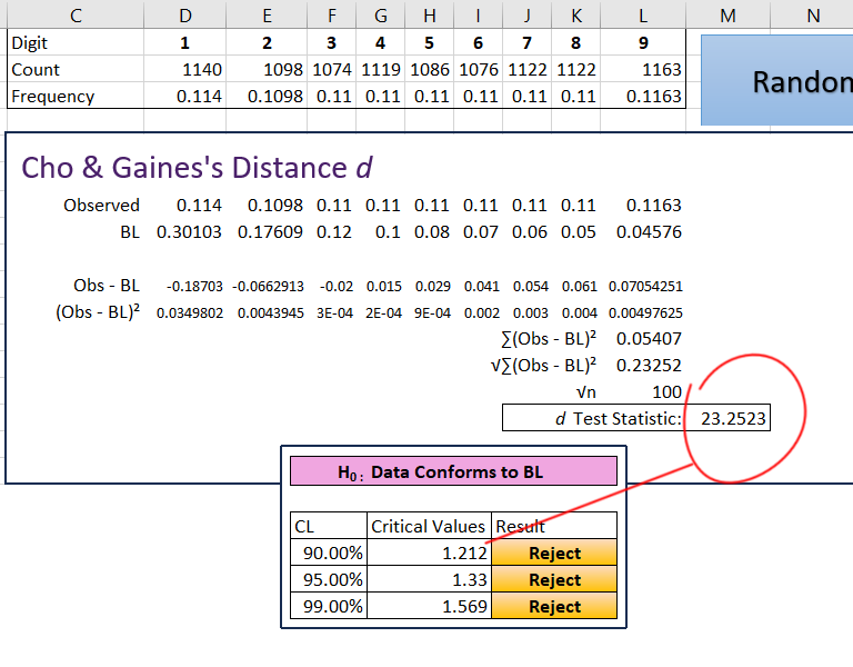
Once again, the test statistic is more extreme than the critical values. The conclusion is the same as for the chi-squared test.
All of the work is now finished. Saving this workbook may be a good idea, in the future, you can simply paste a list of numbers into column A and then all the values for the statistical tests will be automatically calculated allowing you to test any data set for conformity to Benford’s law.
After inspection and testing, it is quite clear that random numbers do not obey Benford’s law. So then, can we create a list of numbers that do? Let us take a look at an exponential population growth model:
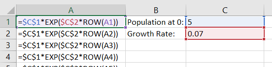
![\[Pop_t = Pop_0 \times e^{r*t}\]](https://lejavbasolutions.com/wp-content/ql-cache/quicklatex.com-f3e00d2fe1f2dc1e61aee6161291c886_l3.png "Rendered by QuickLaTeX.com")
The population at time  is equal to the initial population,
  ,times e raised to the power of the growth rate times the current time period. In Excel we can easily model this:
=Pop0*EXP(RATE*TIME)
Plug those values into the testing spreadsheet and observe:
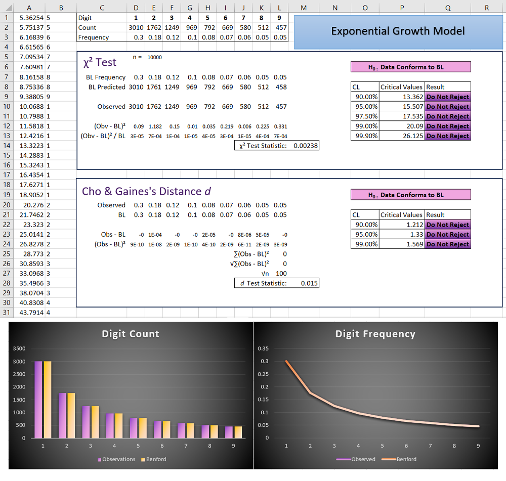
Test Value < Critical Value therefore do not reject
This model appears to strongly conform to Benford’s law. Try changing the parameters: the initial population and rate, it is unlikely that this model will deviate.

After the previous election, these types of graphs came across my social media feeds:
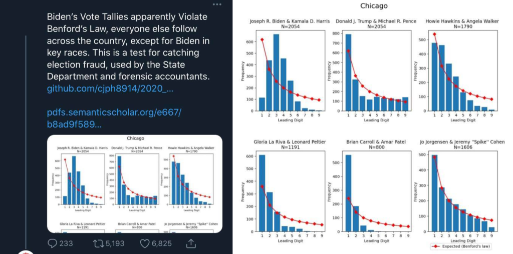
Upon visual inspection, both Biden’s and Trump’s vote totals do not appear to strongly fit the Benford pattern, in violation of the poster’s claim. The proliferation of those posts, as well as many others, seemed to warrant investigation.
As a thought experiment, imagine a city with 5,000 precincts and each precinct holds 1,000 voters (this city is very democratic and sees a 100% voter turnout). This election season, there are two candidates whom are equally popular among the residents. After gathering vote totals, it is a dead tie! Every precinct shows a tally of 500 votes for one candidate and 500 for the other. Without even opening a spreadsheet it is quite clear that listing the data by precinct would simply result in 5,000 rows of the number 500, the first digit frequency would be 0% for all numbers other than 5, and 100% for the number 5. How very un-Benford! In reality, in a tight race, the lead digits would likely bounce around between 4 and 6. If one candidate is heavily favored, then the most common leading digit may be 7, 8, or 9 for them. Allowing for an even more realistic scenario, where the voting population of precinct sizes fluctuates, it becomes even less likely to expect a Benford patten. Further still, precinct sizes are designed to have roughly the same number of people, and they do not span many orders of magnitude, likely into the thousands at most.
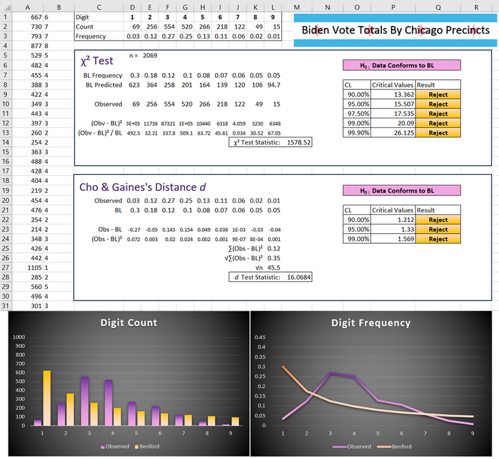
Based on all of the above, the immediate conclusion is that comparing Benford’s law to precinct level vote tallies in Chicago will tell us nothing about fraud. Nonetheless, I performed the tests with data acquired from the Chicago Board of Election Commissioners9.
As expected, the number of registered voters in Chicago precincts do not conform to Benford’s law; the vote totals for each party are not expected to either. Biden’s vote totals do not conform, just as prophesized by the Twitter post, but again, they were never expected to.
Trump’s vote totals:
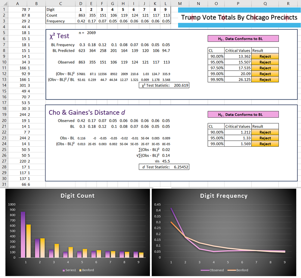
Despite being explicitly told otherwise by the poster, those totals also do not conform, the null hypothesis being rejected at every level.
With a larger data set, and a wider variety of factors involved, county vote totals may be a better candidate for BL analysis. By using data from Harvard10 I have plugged the data into the test sheet:
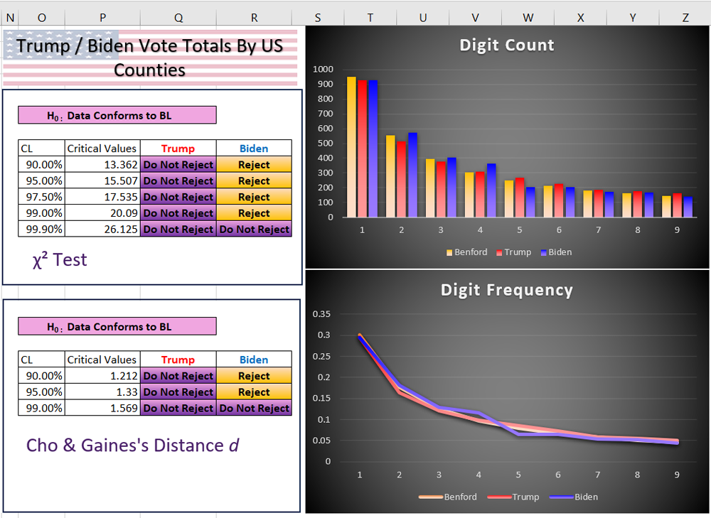
Trump’s vote totals now do exhibit a Benford pattern. Biden’s do not, however we cannot reject the null hypothesis at the highest confidence level, suggesting that it is very, very close to the BL pattern. Nothing looks terribly out of the norm for either candidate, again, in contrast to any claims hastily made on Twitter.
Conclusion
The first conclusion is simple: do not get any important information from internet random people on the internet. However, in order to salvage this from having been an exercise in futility, I believe that there are some important conclusions related to fraud that can be drawn from this analysis.
Those skilled with numbers can use statistics to tell almost any story. There are error bars, confidence levels, and how does one deal with outliers? Which type of regression is appropriate, a ridge regression, or lasso? How many lags in the time series? Which city’s votes mostly appear to violate Benford’s law?
Despite the plethora of avenues available to the econometrician when it comes to choosing how to analyze and present data, there are rigorous rules, checks, and standards. Any intentional falsification, one would hope, would be found during the peer review process, by professionals who know what to look for, wielding tools and knowledge likely unavailable to laymen. Skirting the process entirely, by posting misleading graphs to Facebook for example, may hint at the true intention of the authors.
Chicago must have been chosen because the authors decided, after graphing it, that it was one of the most convincing cities to advance their narrative while completely ignoring the economics of the situation, namely: Committing election fraud is both expensive and risky (not to mention requires, a lot of politically connected individuals to remain quiet about it, perhaps the most Herculean task of all!). It is likely cheaper to simply campaign in any given area to advance your vote totals. Chicago is solidly Democratic. Probably to the point where if Trump won a single precinct, that alone may hint that voter fraud had taken place. I posit that it would be a waste of time and money for any Democratic presidential candidate to attempt to commit fraud in Chicago.
If you have to misrepresent data in order to “prove” fraud, then the only fraudster is you.
- Simon Newcomb, Note on the Frequency of Use of the Different Digits in Natural Numbers, American Journal of Mathematics 4 (1881) 39-40 ↩︎
- https://www.internetworldstats.com/emarketing.htm#google_vignette ↩︎
- https://www.nfl.com/stats/player-stats/category/rushing/2023/reg/all/rushingyards/desc ↩︎
- https://stockanalysis.com/stocks/aapl/revenue/ ↩︎
- Benford, Frank. “The Law of Anomalous Numbers.” Proceedings of the American Philosophical Society 78, no. 4 (1938): 551–72. http://www.jstor.org/stable/984802. ↩︎
- https://mmmcpa.com/blog/theranos-elizabeth-holmes-and-benfords-law/#:~:text=Is%20Benford’s%20Law%20admissible%20in,See%20United%20States%20v. ↩︎
- https://www.politico.com/news/2023/01/25/george-santos-199-expenses-00079334 ↩︎
- John Morrow, 2014. “Benford’s Law, Families of Distributions and a Test Basis,” CEP Discussion Papers dp1291, Centre for Economic Performance, LSE. ↩︎
- Chicago Board of Election Commissioners “Election Results” https://chicagoelections.gov . Last modified February 24, 2024. https://chicagoelections.gov/elections/results/251 ↩︎
- Leip, Dave, 2016, “Dave Leip U.S. Presidential General County Election Results”, https://doi.org/10.7910/DVN/SUCQ52, Harvard Dataverse, V10, UNF:6:h/wB9Gr/kMP46d6KCMW84w== [fileUNF] ↩︎