For this post I will be showing you how to build a dice rolling simulator and, more largely, how to calculate then simulate problems known as “coupon collector” problems, all using Excel and VBA. Starting off with the question, how many rolls of a die would you expect to need in order to roll all six sides at least once? We are going to be essentially proving that statistics works! First we will do some math, then build a dice rolling simulator, then test to see if that math provides an accurate prediction. Let us begin:
The problem: if I have a single die and I want to roll it until I have achieved a roll of 1,2,3,4,5, and 6, how many rolls should I expect to make?
So instinctively we can guess that the minimum amount of rolls required will be 6. That would require the roller to be extremely lucky but it is of course possible. We can also kind of summarize that the upper limit could be extremely high, we can keep rolling the same number, for example, but we can also reasonably assume that the more rolls we make the closer we get to achieving the goal. So what is that number, the expected number of rolls to see every side of the die rolled at least once?
Instead of going into the harmonic series or anything complicated (just yet), lets do it a very simple way using just your basic probability.
The probability of rolling any one specific side of a fair six-sided die is simply 1/6. The expected value of the number of rolls needed to achieve this result is 1 over the probability. So probability is  then the expected value
  is
is ![E[x]=1/(1/6)=6/1](https://lejavbasolutions.com/wp-content/ql-cache/quicklatex.com-9a9508ffbd0d3c6e1656ca352833e783_l3.png "Rendered by QuickLaTeX.com") or just
or just ![E[x]=6/1](https://lejavbasolutions.com/wp-content/ql-cache/quicklatex.com-9d27c678350584002e53d0f5ce08b43f_l3.png "Rendered by QuickLaTeX.com") which equals 6, meaning we expect it to take 6 rolls to get any one specific side of the die.
which equals 6, meaning we expect it to take 6 rolls to get any one specific side of the die.
It follows then that he probability of rolling any 6 of the 6 sided die (not a specific number) is 6/6 or 1. When trying to roll every side of the die at least once, the first roll will always give us a number we haven’t collected yet. The next roll will more than likely give us a new number, the probability is  or
or  meaning we can expect a new number rolled in 1.2 rolls. As we keep rolling and collecting it becomes more likely that we will roll a number that has already been collected, the final number being the hardest to collect with a probability of
  or 6+
or 6+ or just 6, we would expect to roll 6 times in order to obtain the final number. Adding up all the probabilities:
![\[\frac{6} {6} +\frac{6} {5} +\frac{6} {4} +\frac{6} {3} +\frac{6} {2} +\frac{6} {1} = 14.7\]](https://lejavbasolutions.com/wp-content/ql-cache/quicklatex.com-f08c6dee4eb796328681a032283baceb_l3.png "Rendered by QuickLaTeX.com")
To solve the above you can just find the common denominator and you end up with:
720720+864720+1080720+1440720+2160720+4320720
=10584720=14.7
On average, you will need to roll a die about 15 times to get all the numbers pop up at least once. At least that what the math says. Let’s put this to the test by creating a dice rolling simulation and then rolling it a bunch of times. Then we can take the average amount of rolls it took to reach the goal of having every number show up once. Now we can build a simulation and see if it does indeed take an average of 14.7 rolls.


Let me begin by setting up the sheet first, it will look like this when finished:
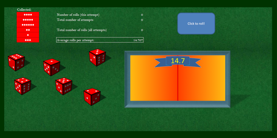
The background is a repeating image of felt that I found online (filtered by license so it was free to alter and use of course, don’t use anyone’s work without permission). The borders are made of an empty rectangle shae filled with a dark green color. The dice I created in GIMP and scattered somewhat randomly on the sheet. The text cells are simply text cells and the values associated with them will be added in later with the VBA. Column B holds six cells that display white dots representing each side of a die. Instead of having the VBA put the numbers collected directly into column B I have it place them in column A and hid them. Column B will display a corresponding number of dots for each number. For example, if there is a 4 in column A then right next to that 4, in column B, there will be 4 dots. The following equation provides that service:
=IF(A3=1,”●”,IF(A3=2,”●●”,IF(A3=3,”●●●”,IF(A3=4,”●●●●”,IF(A3=5,”●●●●●”,”●●●●●●”)))))
However, there is a way cooler and much shorter equation that can be used here as well, the “rept” function. Using that the whole thing is shortened to simply:
=REPT(“●”,A3)
The column holding the numbers, just change the number type to custom and use “” for number type. Color and format the rest as desired.
The graph is a little bit special so I’ll explain it here as well before moving on to the VBA. I want to set up the graph so that the center is the magic number, 14.7, and I want to show a vertical line where the calculated average number of rolls is:
The background is an image I made in GIMP with a red line in the center to indicate the 14.7 value and a banner on top. Double click the plot area, click on fill, then click “Picture or texture fill”. Under picture source click “Insert…” then navigate to your desired image. My graph seemed to work best keeping the number range between 13 and 16.4, so I have a list of those numbers in a separate sheet called “graph data” which is hidden as the user won’t need to see it.
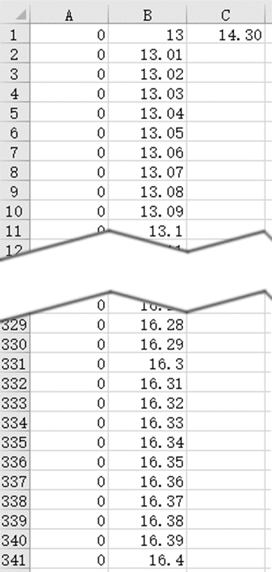
And cell C1 will hold the final average number we are interested in rounded to 2 decimal places. Column A will be the data graphed, it will hold all 0’s except it will hold a 100 next to the average number. So, for example, if average rolls is 14.3 there will be a 100 next to the number 14.3 which is in row 131:
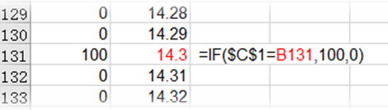
That if statement is very simple, if cell C1 is equal to the cell directly to the right, in this case if cell B131 is equal to C1, then place the number 100 in cell A131, the cell holding the equation. Otherwise it will just place a 0. The vertical line is on a secondary axis with the maximum value set at 100. This way, the line moves across the screen and remains vertical at whichever point it needs to on the horizontal axis.
The VBA
Here is a brief overview of the logic behind the main mechanics then each step will be covered in greater detail and the code broken down by section as well:
- create an array holding numbers 1 to 6
- generate a random number from 1 to 6
- compare that random number to every number in the array
- if the random number is in the array remove that number from the array as it has just been collected
- if the random number is not in the array that means it has been collected before, roll the die again
- once the total number of collected number reaches 6 the program has successfully collected all the numbers
- after collecting all the numbers, check to see if the total number of completions is less than the desired number of completions, if so then reset the simulation and run it again, otherwise end the simulation
Now to set up the routine. The first thing I want this macro to do is hide the cursor. That’s easy, select cell I6, this will hide the cursor behind an image on the sheet. Ok, done moving on to the variables: “times” is the number of times that the simulation has run. It will increase by 1 each time the computer has collected all six sides of the die. “rolls“ will be the number of times the computer had to roll the die to collect all six sides. Define the array I want to use with “Dim arr(5)”, this will create an array with 6 stored values, the “5” in arr(5) may be a little confusing but remember that it includes 0 as a place. So, this array will look like this:
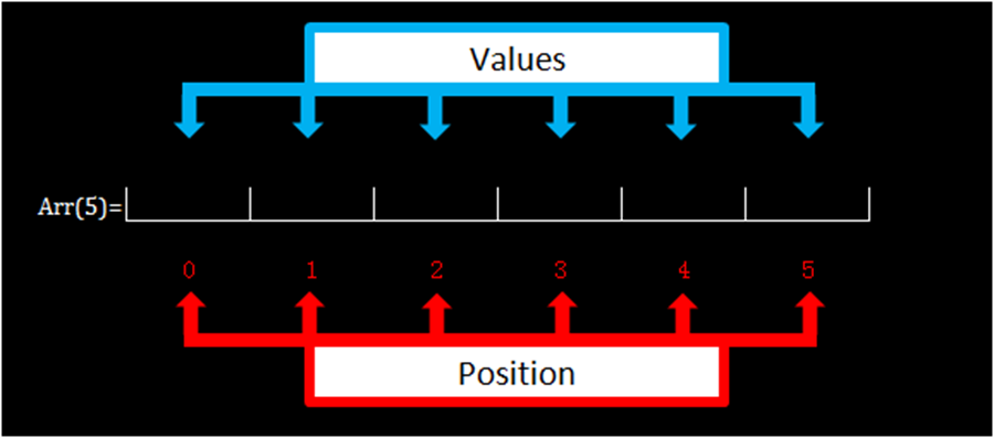
Arr(5) = ””,””,””,””,””,””
Next, there will be three cells holding information, blank those cells before each run by setting their value equal to 0. Everything above can be seen in code form below:
Sub roll()
Range(“I6”).Select
times = 0
rolls = 0
Dim arr(5)
Cells(3, 5).Value = 0
Cells(4, 5).Value = 0
Cells(6, 5).Value = 0
Now, the total amount of times to run the simulation will be entered by the user. Get this value by using in input box and having the user input a number.
totalattempts = Int(Application.InputBox(“Please enter the number of attempts”))
This next step is optional but if the number of attempts is relatively low, less than 1000 say, I will leave the screen updating on and watch the action unfold. If the number is large, greater than 1000, I will turn screen updating off so that it can run through the numbers quicker. Thatis what the following if statement does. If number of attempts (“totalattempts”) is greater than 999 then turn of screen updating, otherwise skip that step.
If totalattempts > 999 Then
Application.ScreenUpdating = False
End If
Now it is time to enter the main loop. This will reset all the values in the array, adding the numbers 1 through 6, and we want to run this loop until all the desired attempts have been played out, so this loop will continue to loop until “times” is greater than “totalattempts”.
Do Until times >= totalattempts
x = 0
r = 1
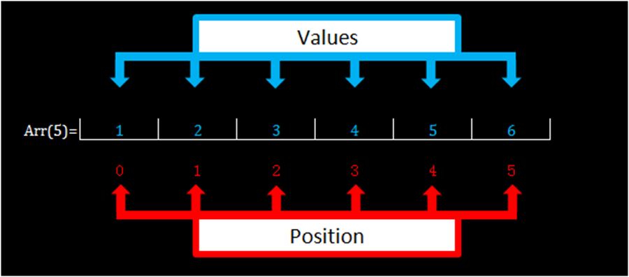
Here we enter a nested loop, all this does is create the array with the proper values. “x” starts at 0 so at position x enter the number x+1. This way, at the very first position in the array, position 0, will hold the number 1 (0+1). Increase x by 1 and then loop again, this time position 1 in the array, the second position in the array, will assume the value of 2 because x+1=2. Do this until arr(5) holds 6 numbers from 1 through 6.
Do Until x > 5
arr(x) = x + 1
x = x + 1
Loop
The above lines of code will set up the array every time we need to rerun the simulation. Now the array has numbers stored in it and it looks like this:
Next, roll the die. This is accomplished by generating a random number from 1 to 6 and you can see the syntax for that below. Check to see if the number just rolled is held in the array or not. If it is present in the array then we haven’t rolled it yet, add it to the list of collected numbers then delete it from the array. If the number we rolled isn’t in the array that means we rolled it before, go back and roll the die again. Every time the die is rolled make sure to increase the variable “rolls” by 1 to keep track of how many rolls it took to achieve the goal.
Do Until r > 6
diceroll = Int((6 – 1 + 1) * Rnd + 1)
rolls = rolls + 1
Here is where we compare the number rolled to every number in the array. As stated above, if it is held in the array then boot it from there and increase the count of collected numbers by 1. If it isn’t in the array simply go back and re-roll the dice.
“y” will be the variable used to check each location in the array so start it at 0 every time and increase it by 1 every time a position is checked. Loop until y is greater than the last place in the array, in this case 5. “diceroll” is the number rolled at random so just compare “diceroll” to every position in the array by using the statement “If diceroll = arr(y) then” and if that statement is true simply kick that number out of the array by setting arr(y) = “” and be sure to increase r by 1 because that means we have added a new number to the collection. Of course, if diceroll does not equal arr(y) then simply increase y by 1 and check the next location in the array. Loop until all positions in the array have been checked. Close that loop and then see if the dice needs to be rolled again. If “r” is still less than the desired total of the numbers we want to collect, for a basic die this is 6, then we have got to roll it again. If r >= 6 then exit that loop as well.
y = 0
Do Until y > 5
If diceroll = arr(y) Then
arr(y) = “”
Cells(r + 2, 1).Value = diceroll
r = r + 1
End If
y = y + 1
Loop
Loop
If the code has made it to this line that means it must have collected all 6 number required because it has just exited that loop. At this point have the program save the total number of rolls it took to get there in a cell, mine is cell (3,5). Increase “times” by 1 because it has just finished another collection attempt. “times” starts off equal to 0 so if this is the first attempt it will indicate that we have successfully collected all six numbers 1 time (0+1).
I also want to get a total of all rolls taken in all attempts and I want that stored in cell (6,5). Cell (6,5) starts equal to 0, add the number of rolls from the previous attempt to this cell using “Cells(6, 5).Value = Cells(6, 5).Value + rolls“ so after 1 attempt this cell will be equal to cell (3,5). Each attempt will see a different number for the “rolls” value in cell (3,5) but cell (6,5) will only every increase as it is a sum of the number of rolls per attempt. Since “rolls” resets every attempt, reset it now with “rolls = 0”. Then close the loop, if “times” is less than the desired number of attempts then the whole process starts again, resetting the values in the array and attempting to collect all 6 numbers again. If “times” is greater than or equal to the desired number of attempts then the loop will break.
Cells(3, 5).Value = rolls
times = times + 1
Cells(4, 5).Value = times
Cells(6, 5).Value = Cells(6, 5).Value + rolls
rolls = 0
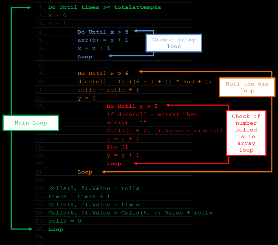
Loop
That’s quite a few loops, here is a handy diagram:
The equation generating the random number can be simplified to diceroll = Int(6* Rnd +1), however the Microsoft manual states that to generate a random number from a range use this: Int((upperbound – lowerbound + 1) * Rnd + lowerbound) so I usually retain the structure to highlight this, and sometimes I will go back and alter the lowerbounds so it is handy for me to do this.
And now to wrap it all up and calculate the average number of rolls. E8 will simply take total number of rolls from all attempts and divide it by the total number of attempts. That will give the average number of rolls it took to collect all 6 numbers. I will then round that number to 2 decimal places and store it in cell C1 on another sheet for the graph mentioned earlier. The graph will pick it up and take care of the rest. Here is the VBA:
Range(“E8”).Value = Range(“E6”).Value / Range(“E4”).Value
Sheets(“graph data”).Cells(1, 3).Value = WorksheetFunction.Round(Sheets(“Dice Roll”).Cells(8, 5).Value, 2)
These next and final lines only concern themselves with showing or hiding two indicator arrows that will appear if my average value is off the graph. The edges of the graph are 13 on the left side and 16.4 on the right side, if the average falls outside this range then an arrow will pop up showing the value and indicating that it is off to the left or right. Those arrows are named “Arrowright” and “Arrowleft”. This is a very simple if statement, if the average value (stored in cell (8,5)) is greater than 16.4 show the right arrow, if the average value is below 13 show the left arrow. If neither of those statements are true then hide both arrows as the line will be visible on the graph. Regardless of whether screen updating was turned off or not, update it and end the sub.
If Cells(8, 5).Value > 16.4 Then
ActiveSheet.Shapes(“Arrowright”).Visible = True
ActiveSheet.Shapes(“Arrowleft”).Visible = False
ElseIf Cells(8, 5).Value < 13 Then
ActiveSheet.Shapes(“Arrowright”).Visible = False
ActiveSheet.Shapes(“Arrowleft”).Visible = True
Else
ActiveSheet.Shapes(“Arrowright”).Visible = False
ActiveSheet.Shapes(“Arrowleft”).Visible = False
End If
Application.ScreenUpdating = True
End Sub
That is all the VBA needed to create a simulator for a specific case of the coupon collector problem. We can alter it a little bit for a more generic approach in the next section.

Before altering the VBA let’s look at the math for the general solution.
Last time we took a quick look at probabilities using numbers 1 to 6, now for the general case of 1 to  .
.
This can take any number of scenarios: in the original example we had a 6 sided die and wanted to roll it until we “collected” all six sides and determined that we expected to roll an average of 14.7 times to collect them all. For another scenario, perhaps there are 10 unique troll dolls hidden at random in the bottom of your favorite cereal, how many boxes would you expect to buy before you have collected them all?
As seen above for the specific case, all we have to do is add up the expected number of tries for each and every collection event. The first collection event will always have a probability of success equal to 1 because we first “coupon” collected will always be a new one.
Let the expected value of each event be ![E[x_k]](https://lejavbasolutions.com/wp-content/ql-cache/quicklatex.com-56549c2f711f1bd35e66449e34421538_l3.png "Rendered by QuickLaTeX.com") with k being the number of the next coupon to be collected. To then get the final number of expected tries, simply sum all of those
with k being the number of the next coupon to be collected. To then get the final number of expected tries, simply sum all of those ![E[x_i]](https://lejavbasolutions.com/wp-content/ql-cache/quicklatex.com-557d64665a0ed694149de2abd710b745_l3.png "Rendered by QuickLaTeX.com") events, so
events, so ![E[X]=E[x_1]+E[x_2]+E[x_3]+…+E[x_n]](https://lejavbasolutions.com/wp-content/ql-cache/quicklatex.com-70d8b7b2c919b733db8f32c9a9575448_l3.png "Rendered by QuickLaTeX.com") . Let’s get that represented by one equation, let
. Let’s get that represented by one equation, let  = the number of the coupon to be collected starting at 1, so begins at 1 and increases by 1 each time a new coupon is collected. For example:
 ![E[x_1]=1, E[x_2]=\frac{n} {n-2+1} , E[x_3]=\frac{n}{n-3+1}](https://lejavbasolutions.com/wp-content/ql-cache/quicklatex.com-c6a87f2d466a8cb6d0b1be6eabe46acd_l3.png "Rendered by QuickLaTeX.com") and so on with
and so on with ![E[x_k]=\frac{n}{n-k+1}](https://lejavbasolutions.com/wp-content/ql-cache/quicklatex.com-f565ac89c19cc18188e58be0c72dc3a3_l3.png "Rendered by QuickLaTeX.com") making the final equation:
making the final equation:
![\[E[X]=\sum_{k=1}^{n} \frac{n}{n-k+1} \]](https://lejavbasolutions.com/wp-content/ql-cache/quicklatex.com-9711137938c7fed9bd05c9349a8755ec_l3.png "Rendered by QuickLaTeX.com")
Plug this equation into Excel and see for yourself, again using the die example:
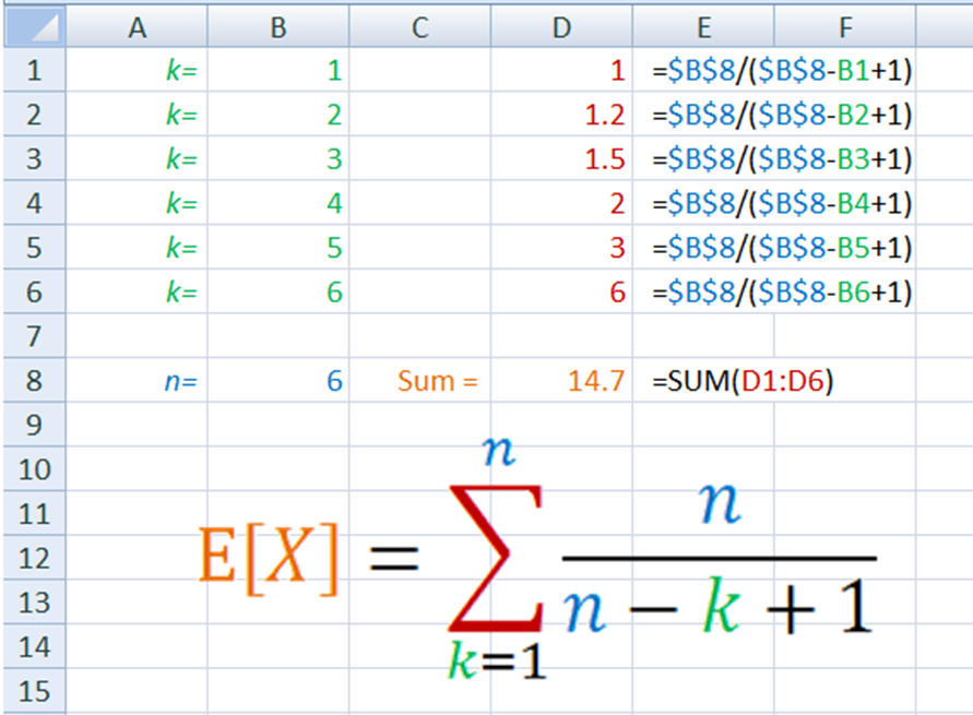
So that is easy enough to see but there is a problem with that equation, it has that sum operator which means that to find very large values of you have to write out all those numbers and then add them up. That ends up becoming very impractical.
What can one do then for those very large values of ? It turns out that those can be approximated using the following equation:
![\[E[X]=H_n \approx n(ln(n)+\gamma)+1/2\]](https://lejavbasolutions.com/wp-content/ql-cache/quicklatex.com-fa85317bb7671b27b7a228c62b8bc374_l3.png "Rendered by QuickLaTeX.com")
With being the number of things to collect and  being the Euler-Mascheroni Constant which is approximately equal to 0.577216.
  is the harmonic number which is the sum of the harmonic series up to .
The harmonic number should look a little familiar at this point. We’ve actually used it above and I can show you how. Take this:
![\[\frac{6}{6}+\frac{6}{5}+\frac{6}{4}+\frac{6}{3}+\frac{6}{2}+\frac{6}{1}\]](https://lejavbasolutions.com/wp-content/ql-cache/quicklatex.com-6232c11cc30a2a6b9873935f2a65b294_l3.png "Rendered by QuickLaTeX.com")
then flip it around, adding the terms with the denominator in ascending order this time instead of the previous way which was by the order of expected value:
![\[\frac{6}{1}+\frac{6}{2}+\frac{6}{3}+\frac{6}{4}+\frac{6}{5}+\frac{6}{6}\]](https://lejavbasolutions.com/wp-content/ql-cache/quicklatex.com-87effff0f1f2436b7e9638f88ceee227_l3.png "Rendered by QuickLaTeX.com")
and factor out the 6 to get:
![\[6*(\frac{1}{1}+\frac{1}{2}+\frac{1}{3}+\frac{1}{4}+\frac{1}{5}+\frac{1}{6})\]](https://lejavbasolutions.com/wp-content/ql-cache/quicklatex.com-92e3c2839848ef2dc9d2afd339829dae_l3.png "Rendered by QuickLaTeX.com")
which is actually 6 times the harmonic series from 1 to 6. So more generally, what we actually calculated for the first section was simply times the harmonic series from 1 to with  which means that the harmonic series was actually there all along just in a slightly different form. We can conclude that:
![\[E[X]=n \times H_n\]](https://lejavbasolutions.com/wp-content/ql-cache/quicklatex.com-22d3d7e0659a1cb7fbce01948bb8d943_l3.png "Rendered by QuickLaTeX.com")
Using the harmonic series like this:
![\[n \times (\frac{1}{1}+\frac{1}{2}+\frac{1}{3}+…+\frac{1}{n})\]](https://lejavbasolutions.com/wp-content/ql-cache/quicklatex.com-0bb06b4222407bbab3eb74094a207d6e_l3.png "Rendered by QuickLaTeX.com")
In plain English, the expected number of tries to complete any coupon collector problem is equal to the number of coupons times the harmonic number of the number of coupons or  where is the number of coupons.
  and
and  and:
and:
![\[nH_n\approx n(ln(n)+\gamma)+\frac{1}{2}\]](https://lejavbasolutions.com/wp-content/ql-cache/quicklatex.com-633ce6655d78e1850fdad62527a0b51f_l3.png "Rendered by QuickLaTeX.com")
That equation is an approximation which becomes more accurate with larger values of . You can play around with this equation as well (I used a with 15 places beyond the decimal point):
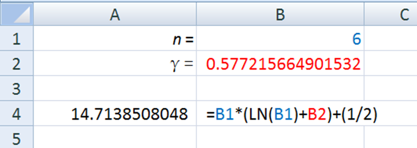
And you will notice that it is close but not exact. For values greater than or equal to 5 this equation is accurate to 1 decimal point and will increase in accuracy as grows. Take a look at  :
:
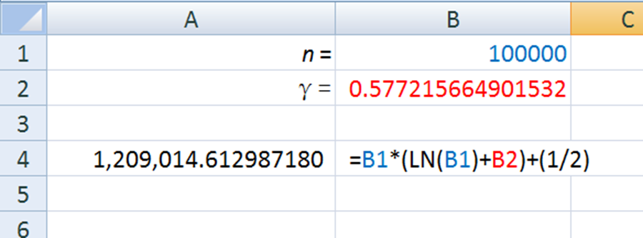
That one is accurate up until 7 places beyond the decimal point.
So that equation enables us to calculate the ![E[X]](https://lejavbasolutions.com/wp-content/ql-cache/quicklatex.com-4249815a79caf7890371efa1a609bb7f_l3.png "Rendered by QuickLaTeX.com") for very large
for very large  without having to calculate, and then then sum over all those numbers. But what about this strange constant? It is worth taking a closer look as to why it is in the above equation.

The Constant in question is in fact the relationship between the harmonic series and the natural log of , specifically it is the limit as goes to infinity of the harmonic series minus the natural log of ,  :
:
![\[\gamma=\lim_{n\to\infty} (\sum_{k=1} {n} -ln(n))\]](https://lejavbasolutions.com/wp-content/ql-cache/quicklatex.com-9256ee263726d2b26ddb4be162c6a28d_l3.png "Rendered by QuickLaTeX.com")
To begin, think about how harmonic numbers are easy to calculate but they have that sum operator in them, making it cumbersome to find the exact values. For large it would be handy to have an equation where one could just plug in and the harmonic number pops out. There currently does not exist such an equation, just the approximate one looked at above. How did that come about and how does the Euler-Mascheroni constant fit in? Well, there is a well understood and well-behaved function that moves with the harmonic numbers and that function is the natural log of . The great mathematician Euler noticed that they move together, hand in hand, as they march off towards infinity. They mimic one another so closely that even though independently they both diverge to infinity, the difference between them stabilizes and actually converges to a specific number. That number is , known as the Euler-Mascheroni constant.
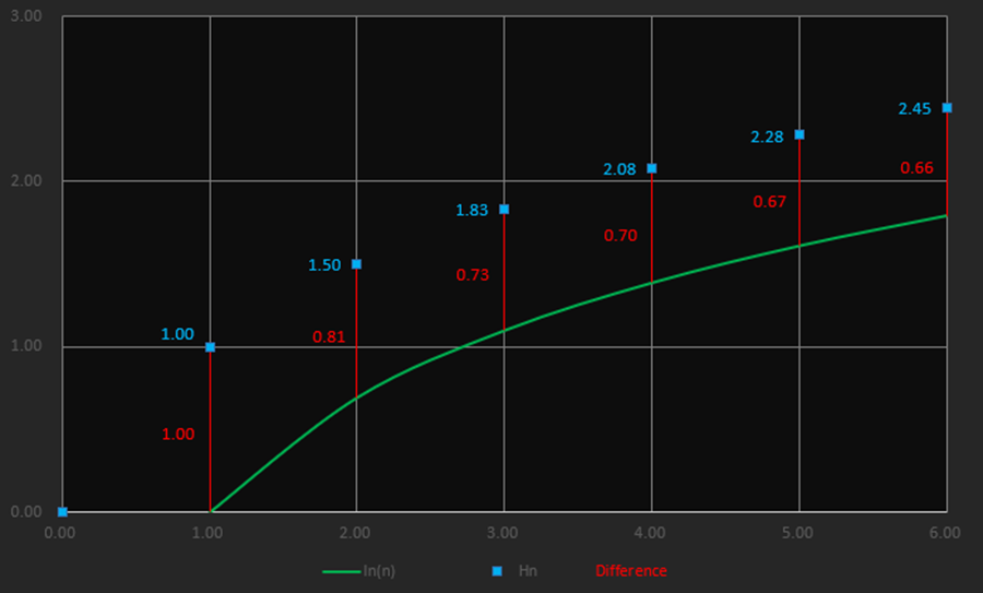
The difference, the numbers in red, will get smaller and smaller until they equal 0.577215…
The harmonic numbers are just a bit larger than the values so all you need to do to estimate is take the value of the natural log of and add .
![\[H_n \approx ln(n) +\gamma\]](https://lejavbasolutions.com/wp-content/ql-cache/quicklatex.com-43969df3392689f3bed94e1b90051b3e_l3.png "Rendered by QuickLaTeX.com")
And one more caveat, remember above where I wrote that the equation is more accurate for larger values of ? Well that’s because the closer to infinity you get the more accurate the approaches the true value of . Which is nice, but both the log function and the harmonic numbers approach infinity really, really slowly. To give it a little kick in the pants mathematicians added an extra term on the equation to make it converge quicker, therefore rendering it a bit more accurate. They added the term  so we can also tack that on the back of ours.
![\[H_n \approx ln(n) + \gamma + \frac{1}{2n}\]](https://lejavbasolutions.com/wp-content/ql-cache/quicklatex.com-1db573c5d9f5f3f3ec2856cbe1923539_l3.png "Rendered by QuickLaTeX.com")
And you might notice, which is pretty cool, that as gets larger the term we added gets smaller because 1 over a large number equals a small number. In fact, at infinity, the end term actually reduces to 0 reducing the whole equation back to  . Neato!
So that’s all well and good except I want a bit more than the harmonic number, I want the harmonic number times . Multiply by and since I did that to the left side be sure to also multiply the right side by .
![\[n \times H_n \approx n\times (ln(n) + \gamma + \frac{1}{2n})\]](https://lejavbasolutions.com/wp-content/ql-cache/quicklatex.com-fd2018d9391ff4561e8afb5bafdbac2b_l3.png "Rendered by QuickLaTeX.com")
![\[nH_n \approx nln(n) + n\gamma +n \frac{1}{2n}\]](https://lejavbasolutions.com/wp-content/ql-cache/quicklatex.com-0771a67e8fe2b4144c90480ab7550594_l3.png "Rendered by QuickLaTeX.com")
And of course the cancel on the rightmost term:
![\[nH_n \approx nln(n) + n\gamma +\frac{1}{2}\]](https://lejavbasolutions.com/wp-content/ql-cache/quicklatex.com-bb596f55dff84dcd86367f00565c631b_l3.png "Rendered by QuickLaTeX.com")
And factor the out to clean it up a bit:
![\[nH_n \approx n(ln(n) + \gamma) +\frac{1}{2}\]](https://lejavbasolutions.com/wp-content/ql-cache/quicklatex.com-5957f1b783a168bce89977a6eeca6e64_l3.png "Rendered by QuickLaTeX.com")
Voila! The equation we used to estimate E[X] from earlier.
One more tangent, I promise, since we now know how important is and what it does, let’s just take a little bit of a closer look at it.
Gamma is defined as:
The integral representation being:
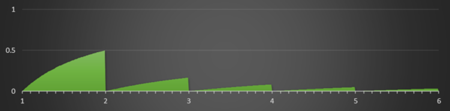
![\[\gamma=\int_{1}^{\infty} \left( \frac{1}{\lfloor x \rfloor} -\frac{1} {x} \right) dx\]](https://lejavbasolutions.com/wp-content/ql-cache/quicklatex.com-af839734fcbfb3e4b49277a39eddabcd_l3.png "Rendered by QuickLaTeX.com")
And what we want is the area between the functions you see graphed there, the area under the bar graphs and above the green line, so all of the blue area.
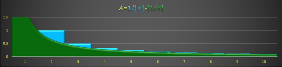
Perhaps this graph is clearer (I don’t usually see it graphed this way but I can see the merits of graphing the whole function together instead of graphing one function minus the other one):
![\[y= \frac{1}{\lfloor x \rfloor} -\frac{1} {x}\]](https://lejavbasolutions.com/wp-content/ql-cache/quicklatex.com-35a295e0dfcd6aca446065a3486afddb_l3.png "Rendered by QuickLaTeX.com")
Solving for the above integral will give us the area. So, take the integral:
![\[\int_{1}^{\infty} \left( \frac{1}{\lfloor x \rfloor} -\frac{1} {x} \right) dx\]](https://lejavbasolutions.com/wp-content/ql-cache/quicklatex.com-afa80740828a37869a987f8cb5757b42_l3.png "Rendered by QuickLaTeX.com")
The integral of sums is equal to the sum of the integrals, so break that bad boy up into two problems:
![\[\int_{1}^{\infty} \frac{1}{\lfloor x \rfloor}dx -\int_{1}^{\infty} \frac{1} {x} dx\]](https://lejavbasolutions.com/wp-content/ql-cache/quicklatex.com-d6c31da1b6c5c93297ed40d5e5299586_l3.png "Rendered by QuickLaTeX.com")
We can solve the right one easier. The integral of 1/x is  (curious, isn’t that? Given that summing over 1/x is the harmonic series and the integral of that is the natural log of x [also, just ignore the end points of the integral for now]):
![\[\int_{1}^{\infty} \frac{1}{\lfloor x \rfloor}dx - ln(x) +c\]](https://lejavbasolutions.com/wp-content/ql-cache/quicklatex.com-11100d615d7beb16b2b30a40a033b0d1_l3.png "Rendered by QuickLaTeX.com")
The integral on the left includes a floor function. So how does one integrate the floor function? It’s actually quite easy but involves using a little trick. The solution may not be obvious at first but two steps will help us get there. One, realize that the integral operator gives us the area under the function. And two, let’s graph the function 
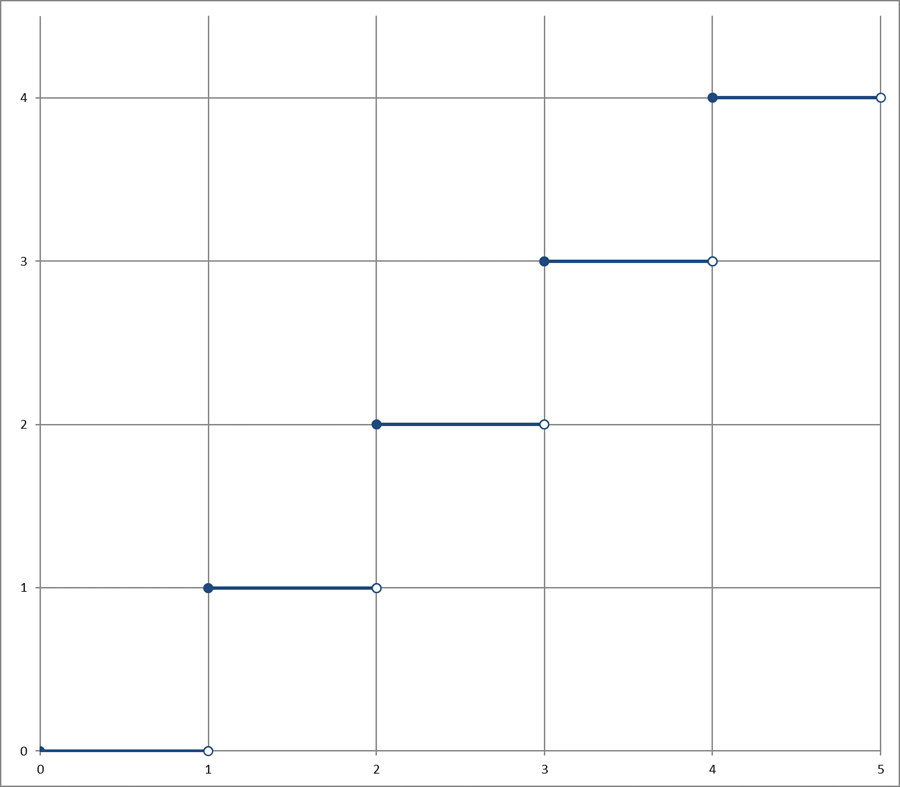
By hand, let’s calculate the area under that function:
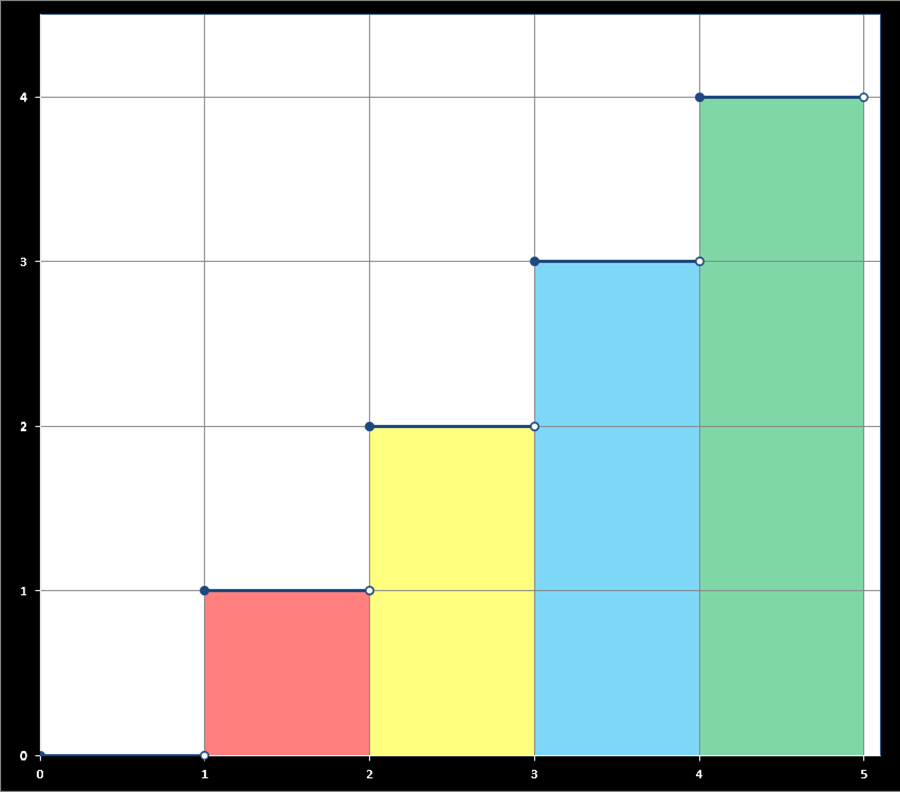
The area from 0 to 1 is 0 as there is no square, the line at the bottom of the graph just moves along at the bottom equal to 0 the whole way. The area from 1 to 2 is the red square, the red square’s area is equal to 1 because the red square is 1 unit wide and 1 unit high so 1 x 1 = 1. The area from 2 to 3, again the area beneath the blue line from 2 to 3, is equal to 2 because there are 2 [1 x 1] squares (the ones in yellow) and so on. Combining areas: the area from 0 to 3 is 3 because that includes that red square and the two yellow squares. The area from 0 to 4 is 6 as there are 6 [1 x 1] squares (red plus yellow plus blue).
So the area from a to b is equal to the sum of areas from a to b-1. We can write that as  and since the integral is equal to the area, we can simply use the sum operator here, ridding us of that pesky integral operator!
![\[\int_{0}^{\n} \lfloor x \rfloordx =\sum_{k=0} ^{n-1}k\]](https://lejavbasolutions.com/wp-content/ql-cache/quicklatex.com-3935649ee27bde7d21417f451139f96d_l3.png "Rendered by QuickLaTeX.com")
And, of course, the integral actually had the term 1 over the floor function which just looks like this:
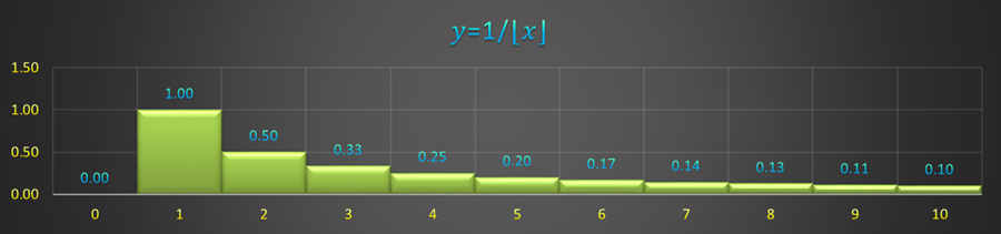
Using the same logic from before, you can see that the area from 1 to 2 is equal to 1. the Area from 2 to 3 is equal to 0.5. The area from 3 to 4 is 0.333¯ and of course you can sum over areas. The area from 0 to 3 is equal to 1.5 and the area from 0 to 4 is equal to 1.8333¯. This means the the area under the curve 1/x is equal to the sum from a to b-1 of 1/k with k being equal to a to b-1. Again, just like before, we can write that out using the sum operator thus eliminating the integral operator.
So:
![\[\int_{0}^{n} \frac{1}{\lfloor x \rfloor}dx =\sum_{k=0} ^{n-1} \frac{1} {k} \]](https://lejavbasolutions.com/wp-content/ql-cache/quicklatex.com-1d922baa7bfd646da9c8555707e1cfe7_l3.png "Rendered by QuickLaTeX.com")
A couple observations as well:
![\[\int_{0}^{1} \frac{1}{\lfloor x \rfloor}dx =0\]](https://lejavbasolutions.com/wp-content/ql-cache/quicklatex.com-e91d9727d2e394f6a0cc11628c554531_l3.png "Rendered by QuickLaTeX.com")
Therefore:
![\[\int_{0}^{\infinity} \frac{1}{\lfloor x \rfloor}dx =\int_{1}^{\infinity} \frac{1}{\lfloor x \rfloor}dx \]](https://lejavbasolutions.com/wp-content/ql-cache/quicklatex.com-5ba09d13c075dc1b18b5b7280bb1dfe1_l3.png "Rendered by QuickLaTeX.com")
Put it together:
\int_{1}^{\infinity} \frac{1}{\lfloor x \rfloor}dx = \lim_{n\to\infty} (\sum_{k=1} {n} -ln(n))\]
Which is the definition of the Euler-Mascheroni Constant.
Finally, how can we be sure about the value of ?
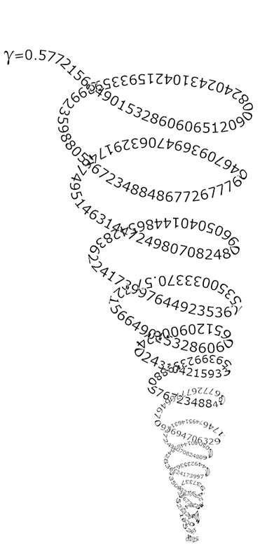
Well, there are a lot of different approaches that have been used to evaluate up to thousands of digits. The most accurate way, probably, is to take the harmonic number of infinity and subtract off the natural log of infinity. We can’t actually do that so I just had Excel calculate the 1,000,000th harmonic number and subtract off the natural log of 1,000,000. This isn’t exact by any means, particularly because Excel can only hold 15 significant digits in each cell, so there is a ton of rounding going on. Nonetheless, I calculated a value of 0.577216164900527, which could be more accurate of course but compared to, say,  , you can see that it grows more accurate as increases.
And that should should just about complete the math portion of this blog post.
That was probably way more than you ever expected to learn about summing probabilities and it was quite a tangent, though hopefully an interesting one. Anyway, without further ado, back to Excel.
Now for the VBA itself:
There will only be a few minor adjustments required to modify the code to our desires. As you may have guessed, the first modification is changing the constant 6 used in the previous example, lets actually turn that 6 into a user entered variable. So the simulation can be altered to collect more than just six numbers, the sky will be the limit! (though, actually, your cpu will dictate the limit). This new variable will be called “arraysize” as that is what technically will change here, if the user wants to simulate a 20 sided die, or a cereal box promotion with 50 different toys, then the array will have to hold 20 or 50 numbers. Grab that variable near the beginning.
arraysize = Int(Application.InputBox(“Please enter the number of coupons”))
The next change will be in defining the array. This new array will no longer be “static,” meaning it will change in size. The size, how many places number it can hold, will be a variable and it will actually be the user input from earlier. To make a “dynamic array,” one that can change size, simply use ReDim instead of Dim when defining it and for the size just use the variable from earlier, I also changed the name of the array to avoid confusion.
From here on out you can just replace every constant 6 with the new variable “arraysize”. The rest will function in the exact same way, the only difference now being that if the user entered a 27 then the dice will keep getting rolled until 27 unique numbers have been collected. Of course, if you are simulating a different scenario than it is that one you can visualize instead of rolling a die, purchasing cereal boxes for example: the program will keep purchasing cereal boxes until 27 unique prizes have been collected. Whatever you fancy!
I have also formatted this sheet a little differently than the sheet dedicated the the dice rolling simulation.
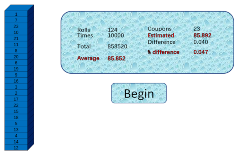
It holds a tower of numbers and has some formatting VBA at the bottom of the code, which you can play with. The main addition is the inclusion of three lines to estimate the ![E[x]](https://lejavbasolutions.com/wp-content/ql-cache/quicklatex.com-397696ada7e139309038cb9b2929e5c5_l3.png "Rendered by QuickLaTeX.com") value:
value:
Gamma = 0.577215664901533
est = arraysize * (WorksheetFunction.Ln(arraysize) + Gamma) + 0.5
Range(“O3”).Value = est
Range(“O2”).Value = arraysize
You should now be able to simulate any size coupon collector problem you desire and compare the results to the expected value of “tries” as obtained by both  and
and ![E[X]=\sum_{k=1}^{n} \frac{n}{n-k+1}](https://lejavbasolutions.com/wp-content/ql-cache/quicklatex.com-0c673cc789ce40a28a8cdc7b86435e10_l3.png "Rendered by QuickLaTeX.com") , allowing a little more understanding as to why these things work the way they do. And of course, the most important thing we have proven, is that statistics actually works and the math very clearly predicts the results, no matter the size of the array, the number of sides on the die, or indeed, the number of unique anythings being collected.
, allowing a little more understanding as to why these things work the way they do. And of course, the most important thing we have proven, is that statistics actually works and the math very clearly predicts the results, no matter the size of the array, the number of sides on the die, or indeed, the number of unique anythings being collected.
Download the spreadsheet below, for whatever reason I can’t upload a xslm file so here is the xlsx file and a text document with the VBA that can be copied and pasted into the VBA module in the spreadsheet.