LOGIT - Leja VBA Solutions

All things will begin with the sigmoid function. Or rather a sigmoid function, as it is a generic term. But it is a function that is bounded between 0 and 1 and is therefore really useful to model binary probability, because an event either happens or doesn’t: you live or die, win or lose, get drafted or not, etc. The function of choice is $\sigma(a)=\frac{1}{1+e^{-a}}$ which, when graphed, looks like the following :

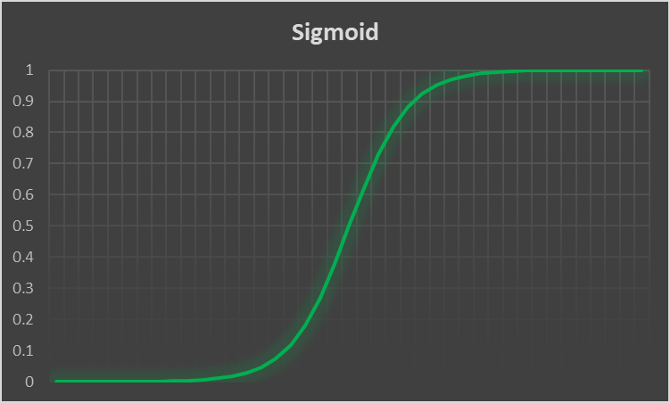
Any point on that line will either really close to a 1 or a 0, and if it happens to fall in that small area in the middle you can consider anything above .5 a 1 and below a 0.5 will be considered a 0.

The idea now is to send our data through this function, and if the end result we get is above 0.5 then we are near the top of the function and consider that to be a 1 (live, win, drafted etc.) and if the result of below 0.5 it is a 0 (dead, lost, not drafted, etc.).

As with linear regression the data will be composed of matrices. The X matrix will hold all of the independent variables, the familiar beta matrix will hold the coefficients or parameters, and the y matrix will be a single column matrix, or vector as they are called, of the 1’s and 0’s. In just about every example and derivation online people use different symbols for the independent variables and parameters but I will use the same ones as linear regression to make things more copacetic and perhaps easier to follow:

$\[\begin{bmatrix} y_{1} \\ y_{2} \\ \vdots \\ y_n \end{bmatrix} = \begin{bmatrix} x_{11} & x_{12} & \cdots & x_{1j} \\ x_{21} & x_{22} & \cdots & x_{2j} \\ \vdots & \vdots & \ddots & \vdots \\ x_{n1} & x_{n2} & \cdots & x_{nj} \end{bmatrix} \times \[\begin{bmatrix} \beta_{1} \\ \beta_{2} \\ \vdots \\ \beta_j \end{bmatrix}$

We can step gingerly through the derivation, sometimes the steps are glossed over too quickly and people may get lost on a step or two, seeing as how we have virtually infinite space on a webpage now, we can time our time.

We will take the log of this, the likelihood expression, and it is easier to work with the negative log, for a lot of reasons that I may or may not elaborate on later, this post is going to be a little long as it is. Anyway, taking the total probability means multiplying the likelihoods together like so:

$\prod_{i=1}^{n} \alpha_i^{y_i} (1-\alpha_i)^{1-y_i}$

What is pretty cool about the above structure is that the first expression is raised to the power $y$ while being multiplied by another expression raised to the power $1-y$ . Recall that $y$ is exclusively either 1 or 0, so when $y$ is 0 then the first expression is raised to the $0th$ power, anything to the $0th$ power simply becomes 1, so that means the first expression is 1 and all that remains is the $1-\alpha$ . If $y$ is 1 then the first expression remains unchanged and the second one, to the power $1-1$ , is now raised to the power 0. Thereby leaving only the first expression. Neat! Anyway, we want to take the negative log of that, resulting in a loss function, then we shall minimize the cost function, which maximizes the likelihood function.

Recall that taking the log of things which are multiplied together results in them being added:

$\log(ab) = log(a) + log(b)$

So:

$-log \left( \prod_{i=1}^{n} \alpha_i^{y_i} (1-\alpha_i)^{1-y_i} \right) = -\sum_{i=1}^{n} log(\alpha_i^{y_i}) + log\left((1-\alpha_i)^{(1-y_i)}\right)$

And by the property:

$\log(a^b) = b*log(a)$

We have the following function I have called $\mathcal{L}$ :

$\mathcal{L} = -\sum_{i=1}^{n} y_ilog(\alpha_i) + (1-y_i)log(1-\alpha_i)$

We will be taking a partial derivative of the above function with respect to the parameter $\beta_j$ since those are of interest to us. And we use $\beta_j$ since we want to take each of the parameters and multiply them by each of the coulmns of the regression matrix. Normally we could take each row of the beta matrix but we are using it’s transpose, so we take the columns “j”. So, step by step, we begin by introducing the partial derivative operator:

$\frac{\partial \mathcal{L}}{\partial \beta_j} = -\sum_{i=1}^{n} \left[ y_i \frac{\partial}{\partial \beta}log(\alpha_i) + (1-y_i)\frac{\partial}{\partial \beta}log(1-\alpha_i)\right]$

Let’s take the derivative one at a time starting with $\frac{\partial}{\partial \beta}log(\alpha_i)$ and expanding the $\alpha$ into it’s true form, $\frac{1}{1+e^{-\beta'x_i}}$ :

$\frac{\partial}{\partial \beta}log(\frac{1}{1+e^{-\beta'x_i}})$

By the log rule:

$log(\frac{a}{b}) = log(a) - log(b)$

We have:

$\frac{\partial}{\partial \beta_j}log(1) - \frac{\partial}{\partial \beta}log({1+e^{-\beta'x_i}})$

The derivative of the log of 1 all goes to 0, the log of 1 is 0 so the derivative would also be 0, then we can apply the following rule to the second part: $\frac{d}{dx} log(f(x)) = f'(x)/f(x)$

$\frac{\partial}{\partial \beta_j}({1+e^{-\beta'x_i}}) = -x_je^{-\beta'x_i}$

Therefore:

$\frac{\partial}{\partial \beta_j}log(1) - \frac{\partial}{\partial \beta_j}log({1+e^{-\beta'x_i}}) = \frac{x_je^{-\beta'x_i}}{(1+e^{-\beta'x_i})}}$

Factoring our the $x_i$ gives us $x_i\frac{e^{-\beta'x_i}}{(1+e^{-\beta'x_i})}}$ and after some algebraic manipulation it can be shown that this is equal to $x_j(1-\alpha)$ .

What we now have is the following:

$-\sum_{i=1}^{n} \left[ y_i x_i (1- \alpha_i) + (1-y_i)\frac{\partial}{\partial \beta}log(1-\alpha_i)\right]$

Let’s work on the next derivative, and there’s a pretty cool trip we can employ here. Recall that earlier we saw that:

$(1-\alpha) = \frac{e^{-\beta'x_i}}{(1+e^{-\beta'x_i})}}$

Rewriting then:

$\frac{\partial}{\partial \beta}log(1-\alpha_i) = \frac{\partial}{\partial \beta}log\frac{e^{-\beta'x_i}}{(1+e^{-\beta'x_i})}}$

And by log rule 2:

$\frac{\partial}{\partial \beta}log(e^{-\beta'x_i})+log(1+e^{-\beta'x_i})$

The $log(e^x)$ cancels the log and the e so now we have:

$\frac{\partial}{\partial \beta}-\beta'x_i+log(1+e^{-\beta'x_i})$

The derivative of the first term leaves us with:

$x_i+\frac{\partial}{\partial \beta}log(1+e^{-\beta'x_i})$

And we just earlier took that exact derivative! So let’s just plug that one in and off we go.

$\frac{\partial}{\partial \beta}log(e^{-\beta'x_i})+log(1+e^{-\beta'x_i}) = -x_i+x_i\frac{e^{-\beta'x_i}}{(1+e^{-\beta'x_i})}}$

Which leaves us now at this point:

$-\sum_{i=1}^{n} \left[ y_i x_i (1- \alpha_i) + (1-y_i)(-x_i+x_i\frac{e^{-\beta'x_i}}{(1+e^{-\beta'x_i})}})\right]$

$-\sum_{i=1}^{n} \left[ y_i x_i (1- \alpha_i) + (1-y_i)(-x_i+x_i(1-\alpha))\right]$

Factor in the x on the far right:

$-\sum_{i=1}^{n} \left[ y_i x_i (1- \alpha_i) + (1-y_i)(-x_i+x_i-x_i\alpha)\right]$

Cancel like terms, also on the right:

$-\sum_{i=1}^{n} \left[ y_i x_i (1- \alpha_i) + (1-y_i)(-x_i\alpha)\right]$

Multiply everything in the parenthesis so ew can start canceling terms again:

$-\sum_{i=1}^{n} \left[ y_i x_i- y_i x_i\alpha_i -x_i\alpha + y_ix_i\alpha_i\right]$

$-\sum_{i=1}^{n} \left[ y_i x_i -x_i\alpha \right]$

Factor out an x:

$-\sum_{i=1}^{n} \left[ x_i(y_i -\alpha) \right]$

And finally factor out a -1 to make it all positive and we have found the derivative that we were looking for!:

$\frac{\partial \mathcal{L}}{\partial \beta_j} = \sum_{i=1}^{n} x_{ij}(\alpha-y_i)$

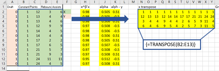
So that looks pretty good, and simple, but I will be using matrix multiplication in Excel and I want things neat and tidy in matrix notation, is there another way to write the above in a linear form? Well, yes. Consider that the above is multiplying a vector $\alpha - y$ times each element in the row of the regression matrix. Lets simply remove the subscripts and the sum operator and write it using matrices instead:

$(\alpha - Y)'X$

And take the transpose of that to give us a nice, clean, vector of parameters.

$\left((\alpha - Y)'X\right)' = \[X'(\alpha - Y)$

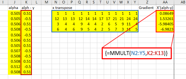
Finally revealing our gradient, which is easy to calculate over the values back in Excel, viola!

$\nabla_\beta\mathcal{L} = X'(\alpha - Y)$

In order to complete Newton’s Method we will need the second derivative of the original function, which, luckily, is simply the derivative of the derivative, and we have just solved that part. So this will be easier, thankfully derivatives tend to get simpler as you continue them (but not always!). Note again, that the second order partial derivative matrix is called the Hessian. So we will technically be computing the Hessian now. So we can take this:

$\frac{\partial }{\partial \beta_k}\sum_{i=1}^{n} x_{ij}(\alpha-y_i)$

Luckily, the only thing in that expression that requires any kind of calculation is the $\alpha$ in there, as that is the only term with any $\betas$ in it. Lets do a little rewrite:

$\sum_{i=1}^{n} x_{ij} \frac{\partial }{\partial \beta_k}(\alpha-y_i)$

$\sum_{i=1}^{n} x_{ij} \frac{\partial }{\partial \beta_k}\alpha-\frac{\partial }{\partial \beta_k}y_i$

And whats nice is that this term $-\frac{\partial }{\partial \beta_k}y_i$ evaluates to 0 so we really only need to calculate the derivative of $\alpha$ and good news, everyone! We can use this cool trick!

Check this out: earlier, we took the derivative of the log of $\alpha$ , so can we use that in order to short-cut our way to the derivavtive of this? Absolutley! The derivavtive of the log of $\alpha$ is as follows:

$\frac{\partial}{\partial \beta} log(\alpha) = \frac{ \frac{\partial}{\partial \beta} \alpha}{\alpha}$

Simply multiply both sides by $\alpha$ and the ones on the right will cancel:

$\alpha \frac{\partial}{\partial \beta} log(\alpha) = \frac{ \frac{\partial}{\partial \beta} \alpha}{\alpha} \alpha$

$\alpha \frac{\partial}{\partial \beta} log(\alpha) = \frac{\partial}{\partial \beta} \alpha}$

And, earlier, we have already taken the derivavtive of the log and alpha and determined it to be $x_j(1-\alpha)$ making the whole expression below:

$\alpha x_j(1-\alpha) = \frac{\partial}{\partial \beta} \alpha}$

So, in a lot of backwards way, we’ve taken that derivative as well, awesome! Let’s plug it in:

$\sum x_{ij} x_{ik} \alpha_i(1-\alpha_i)$

Rearrangeing:

$\sum x_{ij} \alpha_i(1-\alpha_i) x_{ik}$

And that, right there, is the second derivative of the original function.

This is in index notation, but you can kind of see that we’ve got the rows of the matrix times the columns of the matrix times another thing, the alpha time 1-alpha. Well, it turns out, this is something known as a quadratic form, and you can expand it and wrote it all out, but when you have a quadratic form like this, you can make it look much neater by rewriting it in matrix notation. Quadratic forms will begin with the transpose of the x matrix, multiplied by a square matrix in the middle, and then multiplied by the columns of the x matrix.

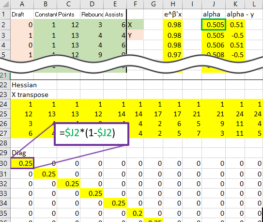
Another thing to note is that we are summing over the $i$ index only, meaning that the alpha matrix will be a diagonal matrix with each element along the diagonal being alpha $i$ times one minus $\alpha_i$ . So the above equation is written more compactly as:

$\nabla^2_\beta \mathcal{L} = X'B_{diag}X$

I would like to add a link to my little matrix calculator soon in order to really elucidate how to move from index notation to matrix notation. I will update this soon when that is finished. For now, let’s just continue using th ematrix notation.

For each step in Newton’s Method you must divide the first derivative by the second, or rather divide the Jacobean by the Hessian, except perhaps you notice that the Hessian matrix is a matrix, as is the Jacobean. So we can’t divide a matrix by a matrix, it’s impossible. Luckily for us, however, we can multiply a matrix by another inverted matrix, which is the equivalent of division. So, as long as the Hessian is invertable, we can do the following:

$(\nabla^2_\beta)^{-1} \nabla_\beta\mathcal{L}$

Assuming the the Hessian can be inverted. If not, there are other methods.

Taken together we can estimate our parameters, $\beta$ , by iterating over a few steps until convergance. That means that we start with some random numbers assigned to the $\betas$ and plug them into the equations.

$\beta_{t+1} = \beta_t - (X'B_{diag}X)^{-1}X'(\alpha - Y)$

Going through all of that yields an nx1 matrix which holds the values for the parameters at each iteration. All that remains is to iterate, again and again and again, until convergence, or until beta t+1 = beta. Awesome! Time to stop peering under the hood of the universe and get back to Excel.

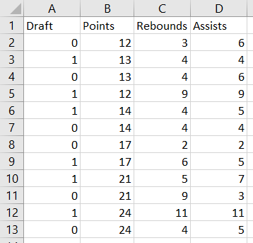
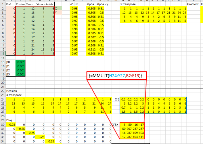
I gathered some data online from this website that I thought was an excellent introduction to how to run a Logit regression in Excel and I would like to mirror the work, except do it by hand using the equations derived above. The sample data is about wether or not a basketball player is drafted based on their previous records. Here is the table:

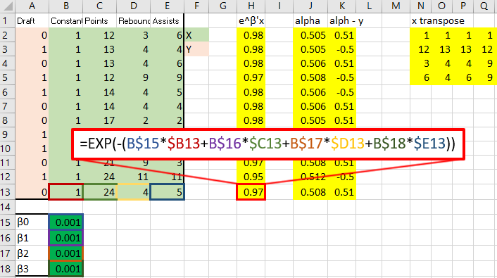
Now, it is only a matter of setting up all the matrix operations that are seen in the equations above. So let’s do that!

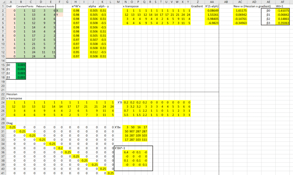
The top right holds the data as well as initial estimates for the $\beta s$ , which I just plugged in as .001. Next to that I have computed the gradient. Below all that I have computed the Hessian. On the right, the two are multiplied to produce the new estimates.

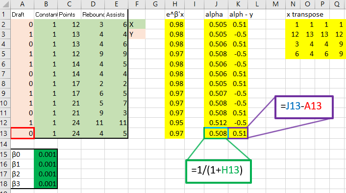
That red box above is the gradient. Now, for the Hessian. Starting with the diagonal matrix, it is simply the alpha value times one minus the alpha value. Alpha one is in cell 1,1 and alpha 2 is in cell 2,2 etc.

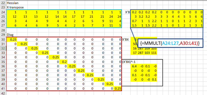
Calculate X transpose times the diagonal matrix B times X:

Then invert it:

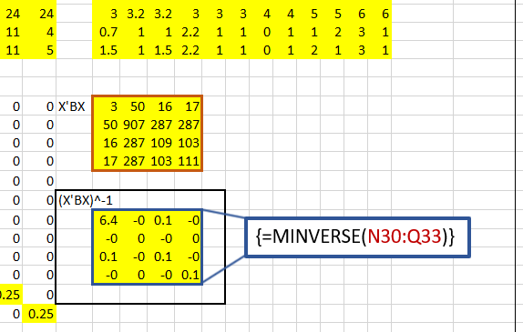
That inverted matrix is the invert Hessian, which can finally be premultiplied to the gradient, revealing the estimates!

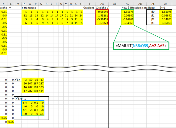
Time to iterate, subract the new $\beta s$ from the original, in this case the original guess of .001:

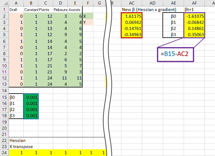
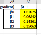
The first thing to notice would be the new estimates, these guys:

And at the moment we can’t be sure if they are optimized or not, perhaps they are what we are looking for, perhaps they are way off. That is normal for now, each iteration of Newton’s Method brings you closer to the optimumzation point, each iteration is a step up the mountain towards the peak. The important thing is that all the equations are set up correctly, then it is simply a matter of copying the sheet a few times and linking the starting $\betas$ back to the previously calculated $\beta s$ like so:

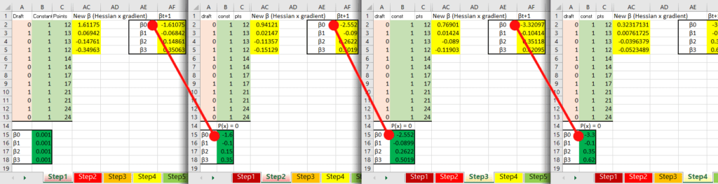
And once the $\beta s$ start to become the same after each iteration, you have reached the optimum point. In math:

$\beta_{t+1} - \beta_t = 0$

After 10 iterations the $\beta s$ don’t seem to be changing much anymore, so we are probably very, very near the optimization point. Let’s take these estimates as final! One more thing to note, we were minimizing which means we were looking for the probability that x was 0, we actually want the opposite, so take the final estimates and multiply them by -1 so we can estimate accuratley.

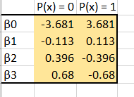
I would encourage you to read the blog I have liked to in order to see how to use solver within Excel to do all the work for you, but I’ll list the values calculated via the solver method here:

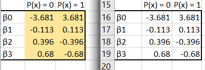
Left: Newton’s Method. Right: Solver Method

And you can see that the estimates match! Congratulations! We have just used Newton’s Method to find the maximum likelihood of a logistic regression extremely manually, (nearly by hand!) and hopefully gained some insight into the real meaning of all those squiggly mathematical symbols. I feel that this exorcise, or experience maybe is a better word, is necessary to really drive home why, and how, these methods work. Equally important is why we can trust them, and knowing when and why they break down and can no longer be trusted. Thank you for working through this with myself, I hope it was enlightening.