Game Theory is a branch of mathematics which economists happen to find very useful. The reason is that Game Theory concerns itself with situations involving some type of competition, or “games,” where players can make moves independent of one another. This setup is analogous to companies, the players, competing for customers, and whichever can gain the most customers wins the “game.” Typically, companies can only position themselves strategically, they can’t do anything to directly hinder the business of their competitors. Well, I suppose they can, but that would usually involve doing something illegal and is generally frowned upon.
Economists will apply game theory to various situations in order to explain why the actors, or players, performed they way they did, and try to explain the world around us as best as they are able. The reason this theory is important is that, as I will explain in this very blog, sometimes rational agents in competition will lead to situations that are sub-optimal. Either for all parties, or for society in general.
The following is a familiar example, though I have not seen it simulated in Excel, so that is what will follow the explanation.
Below we see a picturesque riverfront in a bustling metropolis. Two vendors serve this walkway, they each serve ice cream, snacks, and delicious beer. The residents and tourists can slack their thirsts or satisfy their cravings while taking in the spectacular vista.
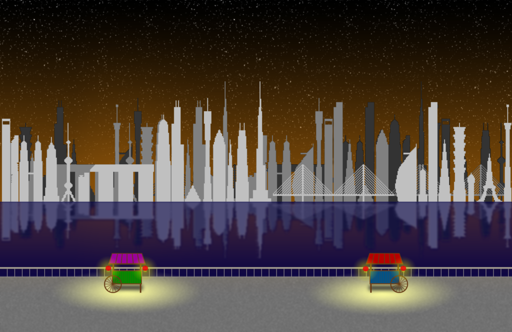
If the walkway is 1 kilometer in length, then each vender is initially positioned so that there exists .5 kilometers between them. Exactly half the length of the walkway. This ensures that half of the territory is serviced by vendor A, and exactly the other half is served by vendor B. Customers can approach at random, from any direction, and will simply purchase from the nearest shop. The “cost” to the customers, aside from the actual cash spend on the items themselves, is the length they must travel. In the initial setup, the maximum length traveled by any given customer is 0.25 km.
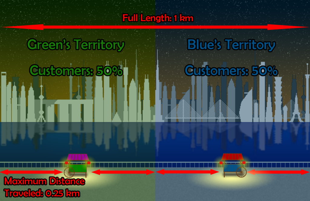
The above is certainly an equilibrium. Each vendor is identical, serves the same amount of customers (on average) and the distance traveled (again, on average) by customers is minimized. This is what is sometimes called a SOS or socially optimal solution. The reason being that should any vendor move their cart any amount in either direction will result in an increase in the maximum travel distance for customers. And it is, as stated, an equilibrium. It is, unfortunately for the customers, not the only equilibrium.
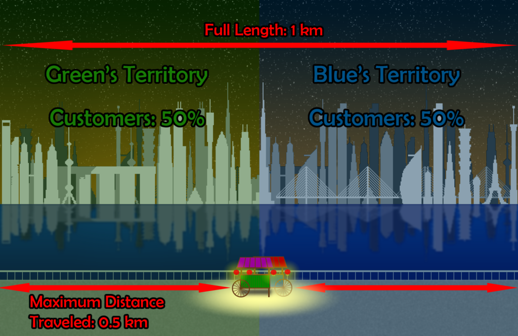
Each vendor can act independently of the other, so, what happens if one decides to move? If vendor A decides one day to move farther from the center, for unknown reasons, then that will give slightly more territory to vendor B. If, more logically, vendor A decides to encroach towards the center, then vendor A still controls all the territory behind them, plus an additional stretch in the middle, potentially stealing customers from vendor B. Vendor B also has the same options, and may also try to encroach on the territory in the middle. Competing over the middle territory will lead to both vendors spiraling towards the center.
Once in the center, there is no unilateral move that either party can take which will make themselves better off. This is a new equilibrium and, likely, won’t change, as there is nothing either party can do to increase customers. This type of equilibrium is called a Nash Equilibrium and is named after the famed mathematician John Nash. Each vendor now claims 50% of the customers, as before, except now the maximum cost for the customers, in terms of distance traveled, has increased to .5 km, or half of the total length of the area. This new equilibrium is not socially optimal. The SOS will never arise again, as neither vendor has any motivation to move from the current location.
Notice, too, that even allowing communication between the vendors, and assuming that the vendors agree not to change the original position, the Nash Equilibrium may still arise. The concept of the chain of suspicion may lead to a Nash Equilibrium and goes as follows.
Vendor A and vendor B agree to not change from the original positions. The penalty for cheating is small, or even insignificant, and the reward for cheater is also small, but greater than the penalty for cheating. Nonetheless, each vendor is very strong in their convictions that the status quo be maintained However, each knows that the other is doing the same calculus; though one vendor has no desire to cheat, they can’t be so sure of the other. The other, also steadfast in its convictions, can have the same suspicions of their opponent. Neither wants to lose, neither wants to cheat, neither knows that the other won’t cheat.
It is very easy to see how unstable the above equilibrium is. Contrast that with the Nash Equilibrium, which we see cannot be broken, and it seems only a matter of time before any system evolves into the Nash Equilibrium, given sufficient time.
First, I would like to calculate the Nash Equilibrium using what’s called a pay off matrix. Then, once we have the theory, I will introduce the simulation, the test of the theory.
To calculate where a Nash Equilibrium exists, create a payoff matrix. This is a grid showing the rewards for each player in every possible position. For this example, there are two player, one player’s payoff is displayed in columns, the other in rows. Combined, it looks like the following:
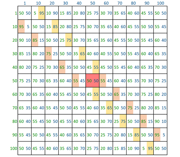
Looking at the grid, or matrix, we can see that if the green player is at position 20, the blue player will choose position 30. This provides the highest payoff for the blue player, based on green’s decision. (Actually, blue’s position would be 21, but I made this grid in 10’s for ease of viewing). If blue moves to position 30, then green will choose position 40 to optimize their revenue. This forces them to continue changing positions until they reach a point where any additional move will result in a decrease in revenue for them. This is the Nash Equilibrium. It is found in the above by simply looking for the maximum number in each column for the column player, and the maximum number in each row for the row player. The cell where they intersect is the Nash Equilibrium and is highlighted in red in the dead center of the above payoff matrix.
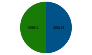
For this simulation, I froze the carts in their initial positions, the green cart in position 26, and the blue cart in position 75. Each simulation consists of 1,000 visiting customers, arriving from random points. And I ran 1,000 simulations for a total of 100,000 customers. As expected, each vendor secured about half of the customers.

| Green Cart | 499,842 |
| Blue Cart | 501,158 |
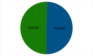
Now, what happens when one morning, a vendor wakes up and realizes that they can encroach slightly into the other vendor’s territory, thereby ensuring that they have a slight edge. Imagine it is the vendor in the left. Any customers arriving from the left edge will always be closer to the left vendor, no matter how far the left vendor moves inward (unless they actually move so far as to cross over the right vendor). However, they will now be able to grab customers who enter from just to the right of the center. A territory previously held by the right vendor. This is signified by the left vendor now controlling an extra column:

Running the simulation again, reveals the results of the skullduggery:
| Green Cart | 505,396 |
| Blue Cart | 494,604 |
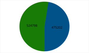
The left vendor sees the results and approves, they move five spaces inward now.

| Green Cart | 524,798 |
| Blue Cart | 475,502 |
The right vendor notices a significant decline in revenue and, upon investigation, realizes that they have lost territory to their competitor. They will copy the same strategy, moving their stall inward as well. This is signified by them moving to the left on the number line, or decreasing the number.

This will continue with each vendor moving closer and closer to the middle.
To see the evolution of the system, each vendor will move in one direction, initially chosen at random, left or right. Next, they will remain fixed for 1,000 customers. After the 1,000 customers each vendor will compare how many customers they served in the most recent iteration to how many they served in the iteration prior. If the number of customers increased, they will move one more space in the same direction as before. This is a reward scenario. If they ended up serving less customers, they will move one space in the opposite direction. The previous move left them worse off.
After sufficient trials, the vendors always tend towards the middle. Usually taking around 150 to 200 iterations to reach convergence. Sometimes they may move in a counterintuitive direction, and they may, through a quirk of random number generating, even be rewarded for it for that iteration. But over time the natural pattern becomes very clear. I have stored each vendors position in the number line after each iteration and created an animation showing how the system evolves.
As well as a graph:
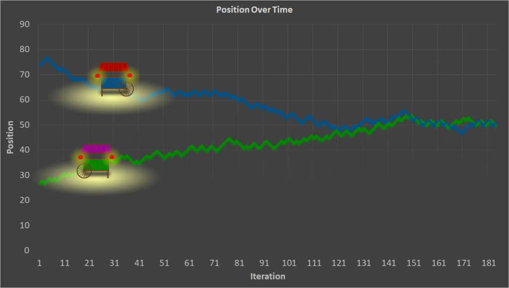
In the above simulation, both vendors converged in the center after around 150 iterations and bounced round the middle zone indefinitely after. Each participant could move in either direction, and we’re perfectly free to deviate from the center. Their actions were simply based on what rewarded the most, and they both refused to leave the middle area. This is very strong evidence of the Nash Equilibrium.
Below is the full code with comments for explanations.
Sub game_theory()
'Starting position for vendor a.
vendora = 26
'Starting position for vendor b.
vendorb = 75
'posa and posb tell each vendor which direction to move in. a 1 indicates a 'shift to the right, a -1, a shift to the left.
posa = 1
posb = 1
'Initialize the customers for vendor a and b.
vendora_old_customers = 0
vendora_customers = 0
vendorb_old_customers = 0
vendorb_customers = 0
'The next variable is the column number that will store the customer location 'data. It starts at column 1
'for the first simulation, column 2 for the second simulation, etc.
customer_column = 1

'Randomly select whether the vendors will move to the left or right.
posa = WorksheetFunction.RandBetween(0, 1)
    If posa = 0 Then posa = -1
posb = WorksheetFunction.RandBetween(0, 1)
    If posb = 0 Then posb = -1

'The main simulation loop, changing the ending number changes how many times 'the simulation is run.
For simulation = 1 To 1000
'The customer loop. How many customers will appear before each vendor adjusts 'their position.
For l = 1 To 1000
'A customers will appear anywhere on the scene, 1 being from the far left, 100 'being from the far right.
customer = WorksheetFunction.RandBetween(1, 100)
'If the customer's location is closer to vendor a, increase vendor a's customer 'count by one.
'That customer will visit vendor a. The same goes for vendor b. If the customer 'is right in the center
'and has an equal chance of of visiting one or the other, use variable LorR to 'give each vendor a 50% chance
'of securing the customer.
    If Abs(customer - vendora) < Abs(customer - vendorb) Then
    vendora_customers = vendora_customers + 1
    ElseIf Abs(customer - vendora) > Abs(customer - vendorb) Then
    vendorb_customers = vendorb_customers + 1
    ElseIf Abs(customer - vendora) = Abs(customer - vendorb) Then
        LorR = WorksheetFunction.RandBetween(1, 2)
        If LorR = 1 Then
        vendora_customers = vendora_customers + 1
        Else
        vendorb_customers = vendorb_customers + 1
        End If
End If

Next l
'Compare the customers from the previous simulation to the current one. If 'this simulation 'resulted in more customers, then the previous move by the 'vendor was a good move. 'They will move in the same direction again as they 'were rewarded. If, however, they lost customers, they will attempt a different 'strategy. To simulate this, reverse their direction of motion by multiplying
'the direction variable by -1.
    If vendora_old_customers > vendora_customers Then
    posa = posa * -1
    End If

    If vendorb_old_customers > vendorb_customers Then
    posb = posb * -1
    End If
'Move each vendor in their preferred direction.
vendora = vendora + posa
vendorb = vendorb + posb
'This round has ended. The current customer numbers will be next round's old 'numbers. The current customer numbers should be reset to 0
vendora_old_customers = vendora_customers
vendorb_old_customers = vendorb_customers
vendora_customers = 0
vendorb_customers = 0
'Take note of the updated locations of the vendors for analysis purposes.
Sheets("Data").Cells(simulation, 1).Value = vendora
Sheets("Data").Cells(simulation, 2).Value = vendorb
'The next round will begin, save the customer data in the next column up.
customer_column = customer_column + 1
Next simulation
End Sub
Are there real life examples of this phenomenon in action? Yes, and it is easily observable in nature. Think of any neighborhood in your own area that specializes in a certain type of business. For example, in Tokyo, there is an area called Shimo-kitazawa, where everyone knows is the best place to go for vintage fashion. And, indeed, there are multitudes upon multitudes of secondhand clothing shops, all in close proximity, sometimes literally on top of one another. In Shanghai, you can have any article of clothing custom made, tailored to your exact specifications, and all the tailors seem to reside just to the west side of Nanpu Bridge. In the US, having gas stations on opposite sides of the road makes sense for ease of cars traveling in opposite directions. Having gas stations on the same side, and right next to each other, seems counterintuitive at first glance, and a mystery to those who haven’t studied economics.
There can be other reasons for the phenomenon, of course, the famous theory of hoteling is a factor here for sure. Hoteling is the idea that businesses will want to be in the center of activity in order to maximize foot traffic, being observed, etc. So businesses in the same industry will research and find the best area of a city to position themselves. Then, within that area, it would make sense for them to spread out, each claiming a small section of the wider area in order to maximize their own customer base while minimizing the travel cost to consumers. This is, of course, not what is observed, as often a competing business will reside right next to it’s competitor. The reason they serve the same geographic area is explained by the hoteling idea, the reason they are nearly on top of one another is explained by John Nash.