Linear Regression in Excel - Leja VBA Solutions

So, you want to run a linear regression in Excel. Maybe you need to do some forecasting, maybe you want to tease out a relationship between two (or more) variables. Maybe you have to explain some phenomenon and predict it, but you don’t have a clue how it works or why it does what it does. These are some of the reasons we run regressions, Excel has a built-in solver feature which does just that, but I would like to build some macros that can also perform regressions, sort of like deconstructing and rebuilding an engine to truly understand how it works. But first, what is a regression?

Before showing the equation, because it may be slightly off putting for those who aren’t terribly fond of math and also because I want to show the intuition first, lets look at a very simple problem: what determines the final score of a soccer game? It’s an easy answer, the number of goals will tell us the final score. Observe how many times a team kicks the ball into the opposite goal and you will know their final score. If each goal were worth 2 points, all you would have to do is multiply the number of goals by 2, but since in this game each goal is worth one you simply multiply each goal by 1 to get the final score. Why multiply by 1? Just to build some intuition, it becomes important later. Now I feel confident enough to write down a simple equation:

Final Score=(Number of goals)×1

Final score is the dependent variable, it is what we are trying to explain. Number of goals is the independent variable, we have no control over it and it is given by observations. 1 is the coefficient on number of goals, we know in this case that it is 1 because everyone knows the rules of soccer, every goal is worth 1 point, if this were football (the American kind) then each touchdown would be worth 6 points so the coefficient on that would be 6. For simplicity we shall stay with the soccer example, let’s make this look a little bit more mathy:

$Fg = Ng* 1$

Got it, but that doesn’t help too much because this implies that we already can explain final score, we can tell anyone the final score if we simply observe the number of goals. Let’s change it so that it looks more like what you will see in real life:

$Fg = Ng* \beta$

There we go, this implies that we believe the final score is a function of one variable (number of goals) times some coefficient (beta). We want to estimate that coefficient, if we can figure it out we can explain our dependent variable, final score. Looking at some data:

Goals	Final Score
1	1
2	2
1	1
3	3
4	4
2	2
3	3
5	5
3	3
4	4
1	1

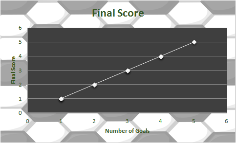
We can be pretty sure that the coefficient is 1, we actually don’t need to run a regression here but let’s look at one anyway:

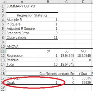
The coefficient on Goals is 1, as expected (I will get into all the other numbers in the future). This brings us back full circle to the equation we started with, our assumption was that the coefficient on goals is equal to 1 and our regression analysis agrees:

$Fg = Ng* 1$

Since the coefficient is 1 we can simply remove it from the equation (anything multiplied by 1 is equal to itself) leaving us with the following equation:

$Fg = Ng$

Final Score is equal to number of goals, easy peasy!

So how about something a little more complicated? Basketball! There are three ways to score in basketball: regular baskets, three-point shots, and free throws from fouls. Let’s set up this equation:

$Fs = \beta_1 * Baskets + \beta_2 * 3-pointers+ \beta_3 * Free throws$

Let’s see if we can estimate how much each of those type of scores are worth.

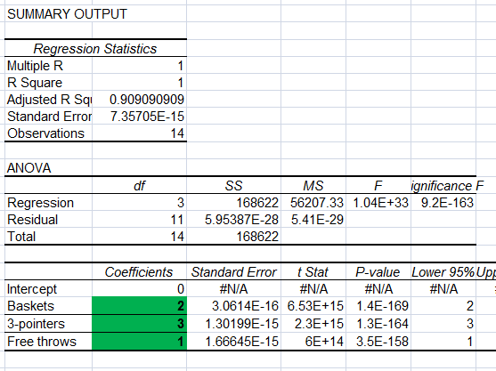
The result of that regression tells us that Baskets are worth 2 points, 3 Pointers are worth 3 points (shocking!), and Free throws are worth 1 point. We can write our final equation like so:

$Fs = 2 * Baskets + 3 * 3-pointers+ 1 * Free throws$

So we have explained how the final score operates and to calculate it all we need to do is observe the number of each type of score, neat!

In the general case we like to use x for the independent variables with a subscript indicating what number they are in the position. Each variable will have a coefficient usually represented by the character beta. And the dependent variable will usually be y so we can substitute y in for Fs:

$y = \beta_1x_1 + \beta_2x_2 + \beta_3x_3$

With y meaning Final score, x1 being Baskets, x2 being 3-pointers, and x3 being Free throws.

Now, if you think about it, it’s pretty interesting that we can actually take a final score and its components and break them up to calculate the value of each component. To see how, I want to look at a single variable regression (single variable with an intercept) in an un-idealized situation (meaning we don’t actually know how many independent variables there are). We can calculate it out step by step in Excel. Then we can look at a regression with multiple variables in an un-idealized scenario and build a macro to run the regression. To complete that final step will require some linear algebra which is just a scary word for matrix algebra. I can’t make it any less scary sounding than that. Hopefully the above example has whetted your appetite to want to learn more.

Simple Regression

The best way to explain how this works is to show a graph, we are trying to explain some phenomenon, y, and we have a ton of data points. Place those data points on a scatter plot and fit a line through that crosses as many points as possible, the slope of that line will be the coefficient on the variable x (only 1 for now).

This should look a little familiar: $y = \beta_0 + \beta_1x_1 + \epsilon$

There are two terms there that I haven’t introduced before, let’s do that now. Thinking back to grammar school, recall that a line can be written with the equation y = mx +b where b is the intercept, the point where the line crosses the y axis and m is the slope. For example:

$y = mx + b$

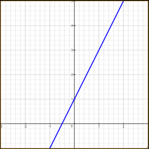
As you can see, the blue line crosses the y-axis at 1. So in the regression the equation for the line will work the same except we usually write the intercept first followed by all the other variables. So we might write the above line like:

$y = \beta_0 + \beta_1x$

And of course $\beta_0$ would be equal to 1 and $\beta_1$ equal to 2

$y = 1+ 2x$

So $\beta_0$ is the intercept (some authors prefer to use the Greek symbol $\alpha$ (alpha) for intercept so you may see that in certain papers or textbooks). The other new term at the end of the top equation is the Greek letter epsilon, $\epsilon$ , which can be called the error term. This term is unobserved and captures all the errors we haven’t accounted for with the independent variables. Let’s use the soccer example again, $\beta_0$ will be equal to 0 because in the absence of any goals final score will be 0. So the line crosses the intercept at 0. The error term will also be 0 because 100% of the dependent variable is explained by the independent variables. The coefficient on any, $\beta_1$ , will of course still be 1. 𝐹𝑠=0+𝑁𝑔∗1+0

You will never see any equation that looks that clean in statistics ever again, in reality you will never even see an error term represented by a number, the error term isn’t observed and it actually needs to be removed from the equation before we make any estimations. This is done using a very basic trick, placing hats on the terms. This denotes that they are estimations and not exact. To expound upon that, consider this equation again:

$y = \beta_0 + \beta_1x_1 + \epsilon$

This exactly explains y and we know this because nothing tells us that these are estimated numbers, further, any variation in y not explained by x will be captured in the error term. So even if x has quite a small influence on y, or we are missing some x observations, all other unseen variables that do influence y will be in the error term. We, however, are seeking to isolate the relationship between known variables so it is necessary to remove the error term. Drop it from the equation but then indicate that these are now estimates by placing hats on the variables like so:

$\hat{y} = \hat{\beta_0} + \hat{\beta_1}x_1$

From now on we will be using this to estimate models, the error term is very important for the theory behind linear regression, and a great deal has been written about it, but in practice we won’t be using it to estimate anything. Let’s work through a real example using the above equation.

Real example

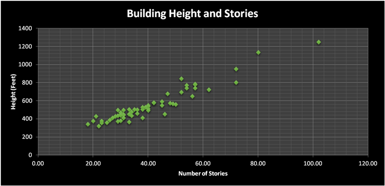
Here is a link to the data we will be playing with, a collection of 60 buildings were surveyed, we have their heights and number of stories.

And here is the equation, we will attempt to estimate the variable “stories” effect of building height. Here is our equation:

��ℎ�^=�0+��×�1

Now let’s finally use Excel. I will have Excel run the regression, we will interpret it, then do it by hand and finally write the macro to do it for us. First you will need the data analysis add-in, then run a simple regression after it is added. Here is the output:

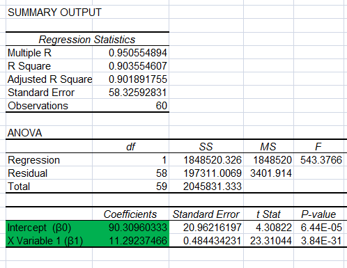
Again, we can explore every number on this output (plus the ones I eliminated for space) but I have highlighted the two I want to focus on here.

Here is a graph of the data, you can see the equation we have estimated right on the graph itself, notice the coefficients are the $\beta_0$ and $\beta_1$ that we estimated:

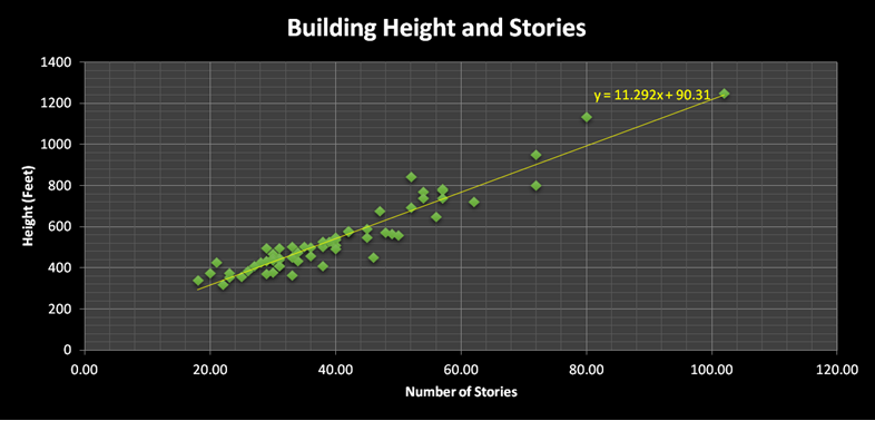
So now that we have the equation it’s time to put it to some use. Pretend that you are in Chicago looking down Lasalle Street and you need to estimate the height of the the Chicago Board of Trade building.

You don’t have the slightest idea how to observe it’s height in feet but you can count the number of windows, vertically, and obtain the approximate number of stories. Some of the windows are longer and some stories near the top look like they may lack windows here or there, so you settle on 44 (there are actually 44 stories but you can see how many you estimate yourself). Once you have the number of stories you can plug that number into the equation and make a prediction about the height:

$Height = 90.309+44*11.292=587$

And that’s pretty darn close! The official height listed here is 574 feet, so our prediction is only off by about 13 feet.

Now that we have seen a regression in action let’s derive those betas.

Here is the theory: we want to create an equation that gives us a y value when we plug in any x value we desire. Ideally, the y value that pops out of the equation is the actual y value observed (emphasis on ideally, you won’t see that outside the soccer example or similar ones). We accept that there are unknown or unaccounted for variables and that we will never estimate an equation which gives precisely the y value listed in the data so we want an equation that gives a value of y closest to the actual observed value of y. The estimated y, the one given by the equation, is called $\hat{y}$ or “y-hat” and the actual y value given in the data is simply called y. We simply want to estimate a y-hat that is close to y, ideally then $y-\hat{y} = 0$ . And again, we accept that that is ideal but not likely. Also, there are many $y$ values in the data so what we actually want is : $y_i-\hat{y_i}$ except we also don’t want a new equation for every $i$ value of $y$ . We desire a single equation that works for predicting all values of $y$ . Therefore to find how accurate the equation is over all values simply take the cumulative effect, sum all y and y-hat values like so:

$\sum_{i=1}^{n}(y_i-\hat{y_i})$

But you may notice the problem there, the equation could be wildly inaccurate and still result in a case where

$\sum_{i=1}^{n}(y_i-\hat{y_i})$

simply because some y-hats are negative and they cancel out y-hats which are positive. To ensure that we have an accurate reading of how close the residuals are you may simply square the residuals like so:

$(y_i-\hat{y_i})^2$

Making the sum of squared residuals:

$\sum_{i=1}^{n}(y_i-\hat{y_i})^2$

Why, then, is the residual squared? Squaring the residuals ensures that each of them will be a positive number (a negative times a negative is a positive). A logical question is then: why not simply take the absolute value? Why square them? And the answer there is that by squaring them the model punishes residuals that are farther away from the trend line. a small residual squared is still a smallish number. A large residual squared becomes much larger. (Consider a residual of 2 which when squared is 4. A residual of 10 when squared is a whopping 100). I want to call this function “S” also known as the sum of squared residuals:

$s = \sum_{i=1}^{n}(y_i-\hat{y_i})^2$

That is the function that we want minimized. In order to minimize a function you take it’s derivative and set it equal to 0. Using this information we can derive the first variable, $\hat{\beta_0}$ :

$\frac{\partial s}{\partial \beta_0} =0$

To take the derivative, multiply the whole thing by the power (2) and reduce the power by one.

$\sum_{i=1}^{n}(2(\hat{y_i} - \hat{\beta_0} - \hat{\beta_1}x_i)) = 0$

Distribute the 2

$\sum_{i=1}^{n}(2\hat{y_i} - 2\hat{\beta_0} - 2\hat{\beta_1}x_i) = 0$

Let’s distribute the sum operator now:

$\sum_{i=1}^{n}2\hat{y_i} - \sum_{i=1}^{n}2\hat{\beta_0} - \sum_{i=1}^{n}2\hat{\beta_1}x_i = 0$

We want to isolate the $\hat{\beta_0}$ so ad $2\hat{beta_1}x_i$ to both sides:

$\sum_{i=1}^{n}2\hat{y_i} - \sum_{i=1}^{n}2\hat{\beta_0} = \sum_{i=1}^{n}2\hat{\beta_1}x_i$

Move the 2’s outside the sum operator since they won’t be effected by it anyway, then divide by 2 to remove all the 2’s:

$\sum_{i=1}^{n}\hat{y_i} - \sum_{i=1}^{n}\hat{\beta_0} = \sum_{i=1}^{n}\hat{\beta_1}x_i$

Subtract $\hat{y_i}$ from both sides:

$-\sum_{i=1}^{n}\hat{\beta_0} = \sum_{i=1}^{n}\hat{\beta_1}x_i - \sum_{i=1}^{n}\hat{y_i}$

Multiply both sides by -1 so that the $\beta_0$ has a positive sign:

$\sum_{i=1}^{n}\hat{\beta_0} = -\sum_{i=1}^{n}\hat{\beta_1}x_i + \sum_{i=1}^{n}\hat{y_i}$

Ad divide by N, the number of observations, so that we can remove the sum operator. Recall that sum of $x_i$ divided by N is actually just the average of $x$ , so we remove the sum operator and denote that it is now an average by adding a bar over the $x$ :

$\frac{\sum_{i=1}^{n}\hat{\beta_0}}{N} = \frac{\sum_{i=1}^{n}\hat{y_i}}{N} - \frac{\sum_{i=1}^{n}\hat{\beta_1}x_i}{N}$

$\hat{\beta_0} = \bar{y} - \hat{\beta_1}\bar{x}$

So we have determined that $\hat{\beta_0}$ is:

$\hat{\beta_0} = \bar{y} - \hat{\beta_1}\bar{x}$

Next we will look at deriving $\hat{\beta_1}$ which is a little more involved but not by too much, we will also be using $\hat{\beta_0}$ , which we just derived, so it is usually best to perform the $\hat{\beta_1}$ derivation second.

So we have determined that:

$\hat{\beta_1}=\frac{\sum_{i=1}^{n} x_iy_i-\bar{y}\sum_{i=1}^{n} x_i}{\sum_{i=1}^{n}x_i^2-\bar{x}\sum_{i=1}^{n} x_i}$

Now that we have the $\beta's$ we can calculate them out by hand and we should get exactly the same values when we had Excel run the regression for us.

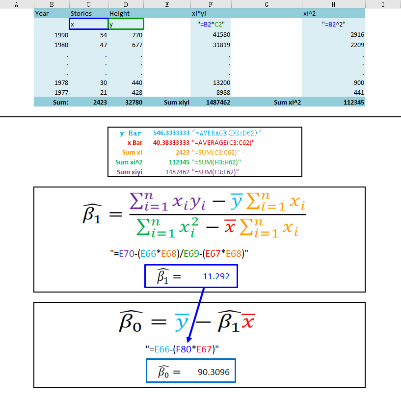
As you can see, we have calculated the exact same values as the Excel add-in and can now run a simple regression by hand, hopeful lending some understanding to these things. Next, I want to write a macro that achieves this for us. After that there will be one more section that looks at some “goodness of fit” statistics, but first, let’s finally do some VBA.

Ok, Let’s define some public variables:

Public headers Public yvar Public xvar Public beta1 Public beta0

Variable “headers” is going to take on a yes or no value (actually a 6 or 7 value), the user will indicate whether or not the data columns have headers. “yvar” will be the column that holds the “y” data and “xvar” wil be the column with our x data. “beta1” and “beta0” will take on the value of $\hat{\beta_1}$ and $\hat{\beta_0}$ .

yvar = UCase(Application.InputBox("Please enter the column letter for the Y variable")) xvar = UCase(Application.InputBox("Please enter the column letter for the X variable")) headers = MsgBox("Does your data have headers?", vbQuestion + vbYesNo) ynum = Range(yvar & 1).Column xnum = Range(xvar & 1).Column lastrow = Cells(Rows.Count, yvar).End(xlUp).Row

As you can see above, the yvar takes a user input as does xvar, if the y data is in column B the user can just type “B” and if the x data is in column “C” then the user can type “C” when prompted. Then, a message will pop up asking the user if their data has headers, this is a yes or no question and headers will take on that value. “ynum” converts the user entered column letter a number. “xnum” does the same except for the x column. Finally, “lastrow” will obtain the number of data rows by obtaining the last row in the column holding any data. Next we will need N, N is the number of observations. In the example using building heights there were 60 years [≈ average human life expectancy at birth, 2011 estimate] of observations so N=60. This will require a slight adjustment depending on whether the data has headings or not. Take a look below:

If headers = 6 Then fr = 2 N = lastrow - 1 Else: fr = 1 N = lastrow End If

Notice that if “headers” = 6 (meaning yes, the data has headers) then the first row of data is row 2, “fr” (for first row) will begin at row 2. Since the data begins at row 2, and row 1 doesn’t count as data, N will have to be the last row of data adjusted down by 1, hence the N = lastrow – 1. If there are no headers than “fr” will begin at row 1 and N will require no adjustment.

Next, assign a variable for all the numbers that we will need to calculate. We must getthe total sum of y, x, the sum x squared, and the sum of x times y. I called these “sumyi”, “sumxi”, “sumxi2”, “sumxiyi”.

sumyi = 0 sumxi = 0 sumxi2 = 0 sumxiyi = 0

Now it is time to build a loop, conceptually, we take a number, say “sumy” and add to itself the value of y from the first row of data, row “fr”. Then, increase “fr” by one row and add that value to “sumy” and so on until all the y’s have been added into “sumy”. Also, note that once we have the total sum of y’s all we need to do to obtain y-bar is to divide by N. Here is that loop:

For r = fr To lastrow sumyi = sumyi + Cells(r, ynum).Value sumxi = sumxi + Cells(r, xnum).Value sumxi2 = sumxi2 + (Cells(r, xnum).Value) ^ 2 sumxiyi = sumxiyi + Cells(r, ynum) * Cells(r, xnum) Next r ybar = sumyi / N xbar = sumxi / N

As you can see above, to get sum xi squared simply square the value of xi before adding it to the “sumxi2” variable. Similiarly, multiply the x value and y value from row r before adding that product to variable “sumxiyi”. Finally, obtain the average value of y and x by dividing “sumyi” and”sumxi” by N and storing the results in “ybar” and “xbar” respectivley. Now we have every number needed to calculate our $\hat{\beta_1}$ which will then allow us to calculate $\hat{\beta_0}$ .

This should actually look a little easier than calculating the betas using formulas, as was shown earlier, because all the numbers have names now so simply plug into the equations from earlier:

$\hat{\beta_1}=\bigg( \sum_{i=1}^{n} x_iy_i-\bar{y}\sum_{i=1}^{n} x_i\bigg) \div \bigg( \sum_{i=1}^{n}x_i^2-\bar{x}\sum_{i=1}^{n} x_i\bigg)$

beta1 = (sumxiyi - (ybar * sumxi)) / (sumxi2 - (xbar * sumxi))

$\hat{\beta_0} = \bar{y} - \hat{\beta_1}\bar{x}$

beta0 = ybar - beta1 * xbar

The only thing left to do now is have Excel spit out the final equation for us, this will take one of two forms depending on if the data has headers or not. If “headers” = 6, meaning yes, then set variable “x” equal to the headers value for the x data column. Same for “y”. If not, simply have “x” equal to “x1” and “y” equal to “y”. Finally, pop up a message box stating the final equation!

If headers = 6 Then x = Sheets("Sheet1").Range("" & xvar & "1").Value y = Sheets("Sheet1").Range("" & yvar & "1").Value Else x = "x1" y = "y" End If MsgBox y & " = " & beta0 & " + " & x & " * " & beta1

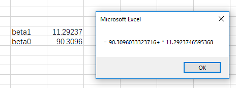
And how cool is that? We created some very simple macros capable of linear regression. The next section will talk about what are known as goodness of fit metrics, SSE, TSS and R squared. I will be revisiting this soon and expounding upon them here (and polishing up the above as well).