I decided to make something a little more practical this time and I also wanted to showcase some VBA required to animate images on the spreadsheet, so I decided to create an animated travel checklist. The VBA used here can have any number of applications for any Excel projects in the future, particularly using images to represent changing data.
This particular project is a simple one, a checklist for travelling. Traveling can be a hectic time, sometimes it is difficult to make sure everything is packed and ready to go, often requires double checking and repacking the night before to make sure that everything is in it’s proper place. So I thought a handy animated checklist might help out. Here is what mine looks like:
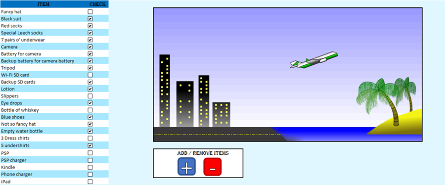
The user creates the checklist and as they complete the items they can check them off. As they check them off the image of the plane begins to take off and once it reaches the right side of the display area a new image will pop up saying “Bon Voyage” or “Congratulations” or something that signifies the list is complete.
It’s a very basic and functional setup. The background is a very light blue, RGB values of 225, 247, 255. Change the font color in columns C and D to match the background, they will hold text that is vital but otherwise messy to look at. Column A holds the item list and the first cell is the header. Column B will hold the checkboxes and has a header as well. The visual area is to the right and I simply filled the bottom two rows of the area in with a grey and used a yellow dotted border to simulate a runway. The blue sky gradient was created using this macro:
Sub colorblue()
Var = 250
r = 18
blue = 255
red = Var
green = Var
Do Until r = 1
Range(“E” & r & “:P” & r).Interior.color = RGB(Var, Var, blue)
Var = Var – 6
r = r – 1
Loop
End Sub
If you want to learn more about colors and gradients and specifically what the above code does you can check out the grow a plant series where I get into colors and gradients a little bit more.
Finally, I added two buttons, one marked “+” and the other “-” they will add or delete items from the list. I’d like to explain those macros first before getting into animating the plane’s flight path.

Cell A1 has my header, called “Items” or whatever you like. First the macro has to ascertain which row to add the new item to. This is fairly easy to do in VBA using the following code.
rownum = Cells(Rows.Count, 1).End(xlUp).Row
Excel will start at the very last row and look for the first row above it that has anything in the cell. For an empty list, this means row 1. We don’t want to overwrite what is in the last row because it will either be holding an item or, in the case of an empty list, the header, so add 1 to the row variable and that should correspond to the first empty row in the checklist.
After setting variable “rownum” equal to the next empty row in the list, add the checkbox and link that checkbox to an adjacent cell. Excel would like to know the position and size of the checkbox so we tell it to place a new check box into cell(rownum, 2), fitted into the top and left of the cell. The width and height should also match that of cell(rownum, 2) so that it is a perfect fit. That takes care of the positioning, then remove the caption by setting .caption = “”. Link it to the adjacent cell using .LinkedCell = “$C$” & rownum (this places it in the same row but column C, one to the right of B where the checkbox lives). In addition to linking the cell automatically, I want to recalculate the plane’s position every time the list is altered so simply call that macro every time a checkbox is clicked using the “.OnAction” command. Each checkbox should be named so that it can be referenced, and therefore deleted, in the future. The simplest way of doing this is to name each check box after the row it resides in, this ensures that there will be no duplicate names either, meaning Excel won’t be confused if we want to add or delete boxes. Here is all that in VBA:
Sub add_new_item()
rownum = Cells(Rows.Count, 1).End(xlUp).Row + 1
Sheets(“Sheet1”).CheckBoxes.Add(Left:=Cells(rownum, 2).Left, Top:=Cells(rownum, 2).Top, _
Width:=Cells(rownum, 2).Width, Height:=Cells(rownum, 2).Height).Select
With Selection
.Caption = “”
.LinkedCell = “$C$” & rownum
.OnAction = “testmove”
.Name = “box ” & rownum
End With
[Quick tip, if a single line of code runs a bit too long you can use ” _” and continue typing on the line below; Excel will treat it as if it were a single line of code]
In row D have the macro add the equation “=if(C” & rownum & “=TRUE,1,””). When the user checks the box in column B, column C will display “TRUE” and column D will display “1” as per the equation we had entered into it. If the user unchecks the item then column C will display “FALSE” and column D will display a blank cell. That is why I reccomended “hiding” the text by making it the same color as the background. Finally, select the new item’s cell in column A so that the user can begin typing right away, replacing the place-holding text.
Cells(rownum, 4).Formula = “=IF(C” & rownum & “=TRUE,1,””””)”
Cells(rownum, 1).Value = “New Item”
Cells(rownum, 1).Select
The equation is important because the number of 1’s in that column will be added up and then compared to the number of items in the list giving us the percentage of the list hat has been completed. That in turn will tell the program exactly where the plane’s location ought to be.
Finally, it is important to format each new item in the list. I chose an alternating pattern between white and light blue. All the program has to do is inspect the row above itself. If the above row is white then the new item’s cells should be light blue. If the above row is not white then make the new item’s cells white. Easy peasy.
If Cells(rownum – 1, 1).Interior.color = RGB(255, 255, 255) Then
Range(“A” & rownum & “:B” & rownum).Interior.color = RGB(167, 232, 255)
Else
Range(“A” & rownum & “:B” & rownum).Interior.color = RGB(255, 255, 255)
End If
I also want to place a line underneath the final item in the list, just to really signify the end. Since we are adding a new item we can be sure that the one above it has a line running along it’s bottom edge. Well, that cell’s bottom is the new one’s top so with the new item’s cells make the top edge borderless and place a border on the bottom edge.
Range(“A” & rownum & “:B” & rownum).Borders(xlEdgeTop).LineStyle = xlNone
Range(“A” & rownum & “:B” & rownum).Borders(xlEdgeBottom).LineStyle = xlContinuous
Here is what we have just created:
There is one final step. Have the macro check that the delete button is visible. I will explain why in the next section. For now, just use another if statement (the button handling deletions will be called “del”):
If ActiveSheet.Shapes.Range(Array(“del”)).Visible = False Then
ActiveSheet.Shapes.Range(Array(“del”)).Visible = True
End If
After all that it is important to recalculate the plane’s position since we have just adjusted the item count. Simply call that macro at the very end.
call plane_position
end sub
The next macro that should be added handles the deletion of items in the checklist. It will almost be the exact opposite of the procedure for adding
items.
Obtain the final row containing any information as before except this time do not add 1 to that number, we actually want the last row. This is the last item on the list so simply blank all the cells associated with it. The checkbox can easily be deleted because we know it’s name, “box” and the row number we are in. Have the macro delete “box “& rownum.
Sub delete_item()
rownum = Cells(Rows.Count, 1).End(xlUp).Row
ActiveSheet.Shapes.Range(Array(“box ” & rownum)).Delete
Cells(rownum, 4).Value = “”
Cells(rownum, 3).Value = “”
Cells(rownum, 1).Value = “”
Cells(rownum – 1, 1).Select
Format the cells in this row back to the background color, remove the border at the bottom of the cells before placing a border along the top of the cells. Remember, the item above will become the new last item on the list so it now requires a bottom border.
Range(“A” & rownum & “:B” & rownum).Interior.color = RGB(225, 247, 255)
Range(“A” & rownum & “:B” & rownum).Borders(xlEdgeBottom).LineStyle = xlNone
Range(“A” & rownum & “:B” & rownum).Borders(xlEdgeTop).LineStyle = xlContinuous
There is a caveat for this sub routine. We don’t want it to delete the headers in row 1. If rownum = 2 we can be sure that we are deleting the only item on the list,leaving behind a blank item list and an item count of 0. If this is the case simply take away the option to delete any further by making the delete button disappear. This is done by setting it’s visibility to false, like so:
If rownum <= 2 Then ActiveSheet.Shapes.Range(Array(“del”)).Visible = False
We can forget about making it reappear because that will happen when the user adds a new item to the list. And, as always, recalculate the plane’s position again after altering the item list.
Call plane_position
End sub
And just in case the item list gets really long, I added a keyboard shortcut for each macro. Ctrl+a is the shortcut for adding items and ctrl+q for removing them.

This macro will be handling where to place the airplane and determining whether or not it needs some rotation. The best way to write this, I found, is to recalculate the plane’s position and rotation each and every time the macro is run based on the number of items and percentage of those items checked in. This way, the plane will be placed in the optimal position whether the user has just checked a box, unchecked a box, added a new item, deleted an item, or accidentally clicked on the plane’s image and somehow flung it into oblivion. It will always pop right back into the position required by the ratio of checked to non-checked items.
Introducing the variables required to make this happen:
Sub plane_position
itemc = WorksheetFunction.CountA(RAnge(“A:A”))-1
Gives the total number of items in the checklist by counting all entries in column A and subtracting 1 for the header to account for the header. After introducing that variable add in this line to handle a specific error. If itemc is 0 then we will get an error if we try to divide by it. Since itemc being 0 represents an empty list anyway just force the macro to exit:
if itemc = 0 then exit sub
Next variable:
chck = WorksheetFunction.Sum(Range(“D:D”))
This adds all the ones in column D, giving us the total number of items marked as completed.
pfin = chck / itemc
Gives the percentage of the checklist that has been completed. We will use that one a lot.
First, let’s look at horizontal motion. The nose of my plane starts in column G and has to continue until it just about touches column Q, in my case this corresponds to a total width of 465 points. So my airplane has to cover an area of 465 points, to determine how much farther along to move it at each after each additional checked item, simply divide 465 by the item count.
This gives you the number of segments that must be traversed by the plane before it reaches the end. That would be the end of it except the plane isn’t starting at the left side of the screen, it is starting somewhere in the middle. In my case the starting position is 330 as measured in points. All you have to do then is add that number to the calculated postion each time and the plane will be adjusted to the right by the correct amount. Use the following equation to achieve all of that:
Plane horizontal position = ((total width / itemc)*chck) + starting position
For example, my starting position is 330 and let’s assume there are 16 items and 8 have been completed:
Plane horizontal position = ((465/16)*8) + 330 = 562.5
The 562.5 minus the starting location is 232.5 which is half of 465. And that is exactly what we would expect the location to be because 8 of the 16 items, or half, have been marked as complete. Code in the horizontal position next like this:
segment = 465 / itemc
hpos = (segment * chck) + 330
Activesheet.Shapes.Range(Array(Picture 2″)).Left = hpos
So, dividing the desired area up into imaginary and equal width columns is easy and you could probably make a similar animated checklist using only that method. A boat, for instance, would only be able to travel horizontally. But this is an airplane so lets make it a little more complicated.
First, the plane will move in a horizontal direction for every iteration, that part is easy and we already looked at the equation. Now I want the plane to also tilt and appear to fly up, following this flight path:
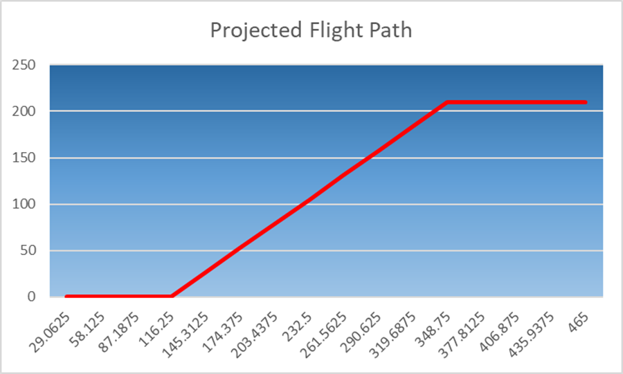
(The numbers on the x axis represent the width of each imaginary column or 465/itemc. 465/16 = 29.0625 so each additional checked item moves the plane by an additional 29.0625)
As you can see from the trajectory graph, the entire vertical area I want to cover is 210 but I only want the plane ascending during the middle portion of the flight. Initially there should be no vertical increase as the plane prepares for takeoff. Then there should be some amount of increase for every additional checked item up until 75% of the items are checked. If a user is checking items and brings the total percent completed to above 75% then there should be no more vertical movement and the plane should rotate back to 0 rotation and continue horizontally.
Let’s tackle the vertical before the rotation. Just as with horizontal movement, we should break up the total vertical space into imaginary rows and use an equation to determine the height of those rows. Assuming a straight, linear flight path we would simply use:
Vertical position = starting v position + (total height / itemc)*chck
Except we want to ascend only during the middle 50% so the equation gets a little messier and needs to be modified.
All we want this equation to do is to get the number of flight segments and height of each segment that are required. So once more than 25% of the checklist has been completed the plane should move upwards 1 segment for each additional item check. For example, if there are 9 items then 25% of 9 is 2.25. If 2 items are checked there should be no vertical movement since 2 < 25% of 9. Once the third item is checked the plane should increase by 1 vertical segment. To get this, decrease the number of checked items (variable “chck”) by 25% of the total items (variable “itemc”). This ensures that it crosses the threshold when we want it to.
vpos = chck – (.25*itemc)
That number gives the number of segments so it should be a whole integer, round it down by taking the integer value of it:
vpos = int(chck – (.25*itemc)
That can now be multiplied by segment height to get the desired vertical position for the plane, however, multiply that number by negative 1 because a smaller number corresponds to a higher position on the sheet and a larger number places the image farther down the sheet. Finally, adjust that number by the starting vertical position, that leaves us with the following:
vposstart = 260
vseg = (210/itemc*.5)
vpos = vseg*-int((chck – (0.25 * itemc))) + vposstart
And we only actually use that position if the number of items checked is between 25 and 75 percent. If below 25% the plane should be locked in at the starting position of 260 and if above 75% the plane should be locked in at the maximum height of 50 points.
So far we have:
If pfin <= (0.25) Then
ActiveSheet.Shapes.Range(Array(“Picture 2”)).Top = 260
ElseIf pfin >= (0.75) Then
ActiveSheet.Shapes.Range(Array(“Picture 2”)).Top = 50
Else
If vpos < 20 Then vpos = 20
ActiveSheet.Shapes.Range(Array(“Picture 2”)).Top = vpos
End If
Now we know how to calculate horizontal position and vertical position for any combination of item list numbers and percent of those items completed. The last piece of the puzzle is image rotation.
While trying to determine the angle of rotation to use for this project I had some fun looking up aircraft take off angles and I found this nifty chart for Beoing aircraft. It was published in this article.
Originally I had set my program to use a 30 degree take off angle but after doing some research I lowered it to 20 degrees, still a bit extreme in the real world but it looks nice for this project. Anyway, onward to the rotations.
To rotate and image using VBA, use this syntax to set the image rotation:
ActiveSheet.Shapes.Range(Array(“My picture’s name”)).Rotation = angle
A negative angle rotates the image counter clockwise and a positive angle rotates it clockwise. So, if I want the plane to achieve an angle of 20 degrees before takeoff I need another equation. Take off is achieved once chck/itemc >= 25% So simply use:
rot = 20 / WorksheetFunction.RoundUp((0.25 * itemc), 0)
to calculate how many degrees of rotation per segment, this one is rounded up because, again, I want whole integers for my segments. I rounded up so that the plane reaches 20 degrees at take off and doesn’t take off while it was still rotated lower, at 18 or 17 degrees or something. Large item lists will result in small degrees per segment and vice versa, this is just like what we did with horizontal and vertical position segments.
Next, to get the desired angle of rotation for an arbitrary amount of items checked off simply multiply the negative of the number of rotation segments by the number of checked items. Again, we have to multiply by a negative because we are rotating the plane counter-clockwise. A positive rotation angle rotates the image in a clockwise motion.
theta = -rot*chck
The above equations will continue to rotate the plane towards 20 degrees until the number of completed items reaches 25%, at which point the plane should achieve an angle of 20 degrees. This equation results in a smooth looking take off angle but it will obviously vary depending on number of items and how evenly things divide into one another. Then, once chck is >25% we can just lock the angle in at 20 degrees until chck reaches 75% and we rotate the plane back to horizontal.
Once the plane is in the final 75% of it’s range it should have already achieved maximum height. There is no longer a need to calculate vpos, simply lock it in at it’s maximum. The angle will have to be adjusted still and it should mirror itself during take off except this time it will straighten out. To adjust the angle here simply take the number of checked items subtracted from the number of total items and multiply that by the rotation segments. This adjusts the angle of rotation down to smaller and smaller degrees until it reaches 0. Add the code handling this upper portion in as well and the final code block should look like this:
If pfin <= (0.25) Then
If theta < -20 Then theta = -20
ActiveSheet.Shapes.Range(Array(“Picture 2”)).Top = 260
ActiveSheet.Shapes.Range(Array(“Picture 2”)).Rotation = theta
ElseIf pfin >= (0.75) Then
theta = -rot * (itemc – chck)
ActiveSheet.Shapes.Range(Array(“Picture 2”)).Rotation = theta
ActiveSheet.Shapes.Range(Array(“Picture 2”)).Top = 50
Else
If vpos < 50 Then vpos = 50
ActiveSheet.Shapes.Range(Array(“Picture 2”)).Top = vpos
ActiveSheet.Shapes.Range(Array(“Picture 2”)).Rotation = -20
End If
A bit verbose in explanation, simple in application.
Now for the grand finale. I created an overlaying image using GIMP that reads “Bon Voyage” and set the transparency quite low. I want this image to pop up over the display area once 100% of the checklist has been completed. This is really easy to do. After creating your image, import it and place in in the desired position in the Excel worksheet. Rename it, I called mine “end”, and just place these lines of code at the end of macro handling plane movements:
If pfin >= 1 Then
ActiveSheet.Shapes.Range(Array(“end”)).Visible = True
End If
This displays your completion image immediately and hide the image if the checklist hasn’t been completed in full.
That should finish off the animated travel checklist. All that’s left to do is book a flight, make a list, then begin checking off items in preparation for your holiday. Happy traveling!