This time we’re looking at something called the Josephus problem. As far as I can tell this is based off of an actual event in history or is at least attributed to a historical figure, Titus Flavius Josephus. Here is the basic set up:
Josephus and 40 other of his fellow Jewish soldiers are surrounded and will imminently be captured by Roman Soldiers. The Jewish Soldiers feel that death is preferable to capture so they devise a system where each member kills another until there is only one left and that person would then commit suicide. So, they all stand in a circle and each person will kill the one to their immediate left. They would keep going around and around until there is only the one left. Now, Josephus was the only one who actually preferred capture to death but, fearing becoming an outcast, he didn’t want to voice his views. Thus, he needed to figure out where exactly in the circle to sit so that he is guaranteed to be the last survivor.
And that is the system we are going to build and analyze in Excel. There are variations of this story, that the procedure was to kill every third person instead of every second and we can actually make our program do that too. But I will start by building a simulation killing every second person and from there it’s simply a matter of adjusting the inputs to whatever we like.
For a more in depth explanation of the problem see this video which does a remarkable job of explaining it.
Just a quick note on the notation, for every time I run a Josephus problem “n” will stand for the number of people in the circle and “K” will be how often a kill is made around the circle. If K = 2 then every other person is killed, if K = 3 then every third person is killed etc.
Part 1: Creating the Simulation
This is what we will be building:
Here is the list of variable declarations first:
Dim n As Long
Dim Pi As Double
Dim picdeli As String
Dim nalive As Integer
Dim rowpos As Integer
Dim colpos As Integer
Dim winner As Integer
Dim viscols As Double
Declare Sub Sleep Lib "kernel32" (ByVal dwMilliseconds As Long)
These will all be explained as they come into play. One that I haven’t used in a blog before is “Sleep” which will allow the program to pause for a given amount of time during execution, I use this for handling the animation in the simulation.
To begin, we have to create a circle of people and set up the view so that the circle is centered in the the spreadsheet. So first I will talk about sub vis, this actually isn’t the first subroutine but it is called right away and sets up the window so it’s best to begin here. The number of people, called “n”, is obtained from a user input earlier. I want some space between each person and I found that the best way to do that is to have the circle of people’s diameter (measured in cells) equal to the number of people in the circle + 1. Also, the circle always starts at the top of the screen, so since I have starting position and diameter I can now figure out how far to zoom out to get the best view of the circle. That is the logic behind this macro, find the bottom of the circle and continually zoom out until the bottom is within view.
The number of rows to be displayed will be called “neededrows” and they will be equal to diameter plus one. Diameter is equal to n + 1 so neededrows will be equal to diameter +1 (or n+2), giving us a row of clearance on top and on bottom.
Next, zoom in to the maximum zoom level, I chose 200, and begin zooming out until the number of needed rows is greater than the number of visible rows. There is a nifty function in VBA that tells you the number of visible rows and I used it below, visrows = ActiveWindow.VisibleRange.Rows.Count.
So to recap, calculate the diameter and add 2 to obtain the number of rows we want visible, zoom in to maximum zoom and simply zoom out until neededrows is greater than visrows.
Sub vis()
Application.ScreenUpdating = False
diam = n + 1
neededrows = diam + 1
zoomers = 200
ActiveWindow.Zoom = zoomers
Do Until visrows > neededrows
visrows = ActiveWindow.VisibleRange.Rows.Count
If zoomers < 10 Then
Exit Sub
End If
ActiveWindow.Zoom = zoomers
zoomers = zoomers - 1
Loop
End Sub
The window is now set and Excel will begin placing the people in a circle. First it will place a person into a cell in numerical order and color the cell green, this signifies that the person is alive. When a person is killed, they turn red. That’s the mechanics of it but I superimposed images over each cell, a smiley face for a living soul and a skull for the recently deceased.
This is where it actually begins. Start by turning off screen updating. Set “Picture” equal to the path where you store the picture you want to use for each living person. Mine is called “smile” and you can see the path below. Next it calls reset which simply resets the previous simulation, we can look at it later.
As you might have guessed, since we are creating a bunch of people standing around in a circle we will need some trig, meaning we will need Pi as well. So make sure you perform the usual Pi = WorksheetFunction.Pi.
The number of people will be up to the user so set n equal to user input using n = Application.InputBox(Promtpt). Now that Excel has the critical n value it can call vis and set up the screen.
Sub rotate()
Application.ScreenUpdating = False
Picture = "C:\Users\Rik7000\Desktop\Ex-Cell games\smile.png"
Call reset
Pi = WorksheetFunction.Pi
n = Application.InputBox("Please enter the number of people")
Call vis
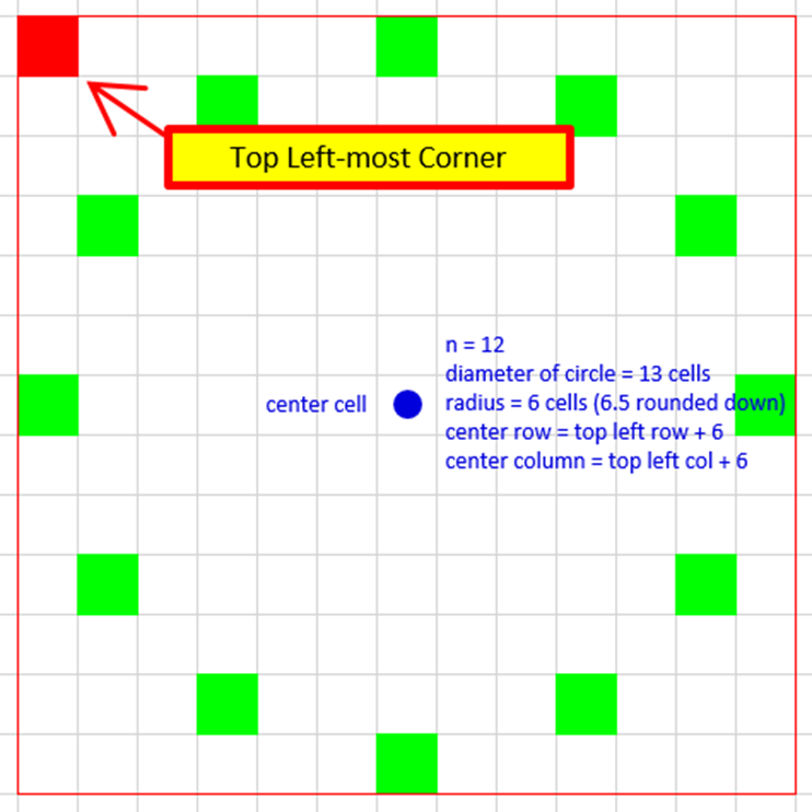
The center of the circle needs to be calculated first. The middle cell’s row is easy, it’s the radius of the circle with diameter n plus 2 (so that the top of the circle is just below the top of the screen). The middle cell’s column will vary based on how wide the circle is, I want it to always be in the center of the screen (except for sufficiently large circles). So grab the number of visible columns and store that in viscols. Grab visrows while we’re at it, we will need it later.
viscols = ActiveWindow.VisibleRange.Columns.Count
visrows = ActiveWindow.VisibleRange.Rows.Count
The column of the center cell must be adjusted. I will store that adjustment value in variable “adjcol” which will be equal to (viscols – n)/2. It takes the number of visible columns and subtracts the diameter of the circle, that gives the number of columns on the screen outside of the circle. Because the circle should be centered divide that number by 2 and the is how far from column 1 the leftmost cell of the circle ought to be. For very large values of n this would actually be unfeasible as the circle would have some people occupying spaces to the left of column 1, which crashes Excel. To get around this, if the adjustment results in just that scenario simply push the center cell’s column value to the right by the needed amount to bring everyone back onto the page. That is what the following loop does:
adjcol = (viscols - n) / 2
If adjcol < 1 Then
Do Until adjcol >= 1
adjcol = adjcol + 1
Loop
End If
rowpos = 2
colpos = 1 + adjcol
After the adjustment is calculated we now know the top-left most position of the circle. To get the actual center of the circle from there simply add the radius to both row and column variables (if n is an odd number Excel will round for you and the center will always work out). You will see that being done below. A bit like this:
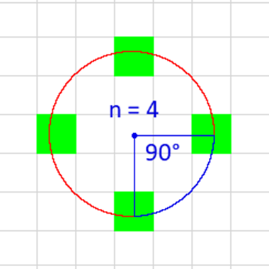
Each person will occupy a cell as determined by a segment of the circle. Each segment is calculated as a fraction of a circle so to get that number, simply divide 360 by n. For example, if n is 4 then each person occupies a place 25% of the way around the circle, so at each 90 degree angle from the origin.
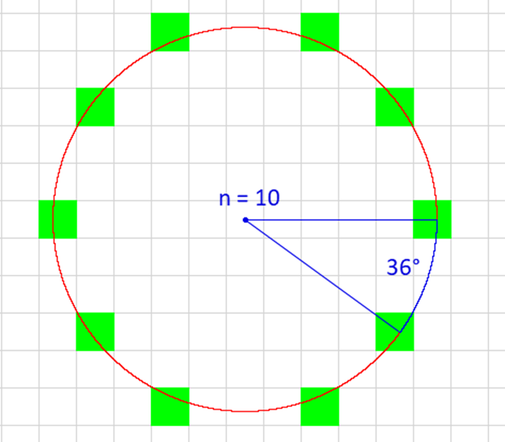
For n equal to 10 then each person occupies a space 36 degrees around the center (360/10 = 36):
And set the loop so that it places a person at each interval starting from 1. Variable “div” (for divisor) will start at 1 and loop until div is greater than n, ensuring everyone gets a seat. The VBA looks like this:
seg = 360 / n
div = 1
Do Until div > n
To get each individual’s segment, which will be translated into row and column coordinates later, divide 360 by (n*div). For the example of n = 4, the first person’s segment number is 360 / (4*1) = 90. Next, take the sine and cosine of 90 which gives 1 and 0 respectively. Next, multiply those numbers by the circle’s radius. Finally, add the radius to those numbers and that is exactly where the first person resides. For example, let diameter = 4 so radius is = (4/2). So for person 1, row value is 1 * (4/2) = 2. That means that person 1’s row will be offset by 2 from the middle cell. The mid point is cell (4,18) meaning the row value for that person is 6. Column value is 0* (4/2) + 18 = 18. So person 1’s column position is 18. Person 1 resides in cell (6,18).
Person 2’s location is determined the same way except now seg is (360/4) * 2 which is 180. the sine and cosine values for 180 will be flipped so now the row offset will be 0 * (4/2), the row offset is 0 and the initial row position is 4 so the final row value for person 2 is 4. Column value = -1 * (4/2) = -2 so the column value is offset from the middle by -2, person 2’s final column value is 16.
Here is a listing of the row and column values for each person if n = 10, hopefully this table helps clear things up a little bit:

Keep in mind the the middle cell’s row value is rowpos + (n/2) and it’s column value is colpos + (n/2), that is where we make the offset from. There is one additional line but all it does is convert seg from degrees to radians so that the trigonometric functions calculate the proper values, that’s all. Call that seg1 and take the sines and cosines from there.
seg = (360 / n) * div
seg1 = (seg / 180) * Pi
y = (Sin(seg1) * (n / 2))
x = (Cos(seg1) * (n / 2))
Cells(rowpos + (n / 2), colpos + (n / 2)).Offset(y, x).Interior.ColorIndex = 4
Cells(rowpos + (n / 2), colpos + (n / 2)).Offset(y, x).Value = div
Set the calculated cell’s value equal to div which is also the seat number and color it green. Next, place a smiley face over it to signify they are alive (it looked a little bit better than just using a green cell). Change the name of the picture over the seat to the value of div as well, this way the user can tell which seat number is which by clicking on the picture and noticing the picture name.
With Cells(rowpos + (n / 2), colpos + (n / 2)).Offset(y, x)
Set mypic = ActiveSheet.Pictures.Insert(Picture)
mypic.Top = .Top
mypic.Left = .Left
mypic.Width = .Width
mypic.Height = .Height
mypic.Name = div
End With
That will place the picture inside the cell and make it the same size as the cell. Next, increase div by one and do it all over again for person 2 up until you have placed all people from 1 to n.
div = div + 1
Loop
Every time this simulation resets it will delete all images on the sheet. This means that every button on the sheet will have to be replaced for every simulation run, but that is no problem! Simply set the “Picture” variable to the new image that will become the button. Mine is called “run simulation.” I want it in cell (1,1) but the size will vary depending on the zoom level set by vis. I want mine about 1 / 8th of the visible columns on my screen in width and about 1/4th of the visible rows in height. Obtain the width and height as seen below. Then its simply a matter of placing and sizing the image as well as adding it’s action, which is to call “rounders” when clicked on.
Picture = "C:\Users\Rik7000\Desktop\Ex-Cell games\run simulation.png"
width1 = Int(viscols / 8)
height1 = Int(visrows / 4)
With Cells(1, 1)
Set mypic = ActiveSheet.Pictures.Insert(Picture)
mypic.Top = .Top
mypic.Left = .Left
mypic.Width = .Width
mypic.Height = .Height
mypic.Name = "rs"
mypic.OnAction = "Module1.rounders"
End With
ActiveSheet.Pictures("rs").Height = Sheet1.Range(Cells(1, 1), Cells(height1, 1)).Height
ActiveSheet.Pictures("rs").Width = Sheet1.Range(Cells(1, 1), Cells(1, width1)).Width
End Sub
After running that there should be a nice circle of smiley faces centered on the sheet as well a button in the top left corner that will start the simulation when clicked. For example, here is n = 17:
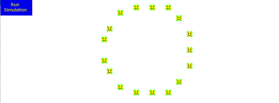
Next we look at how the simulation is actually performed.
Remember how each living person’s cell is green and each dead person’s is red? That will be important here. The images over them won’t be used to calculate anything, they are purely for aesthetics.
This macro will loop around the circle examining each person’s cell using the exact same formula as the previous macro, this ensures that nothing is missed. It will also need a kill countdown programmed into it. As it loops around the circle the count down will decrease by 1 for each living person that is passed. Once the count down is 1 then the program will kill the next living person it sees. Note that it will actually ignore all dead persons, the program simply skips along if it finds a corpse.
Lets look at an example where K = 2, meaning every other person dies. First it will look at person 1 and if the simulation has just started then that person’s cell will be green. The program will not kill them, it is not yet ready to kill but it will decrease K by 1. Now K is equal to 1, meaning the next person will die. The program evaluates person 2’s cell, it is green meaning they are alive. The program kills them, turning their cell red and placing a skull image over it. The kill count down is reset. Person 3 is determined to be alive and the counter ticks downs again, person 4 is alive and is then therefore killed. After one round of this, lets assume that person n-1 has just been killed so now we are back to person 1 with a full kill timer. It will leave 1 alone and decrease the timer moving on to person 2, but person 2 is already dead, the program sees this and simply does nothing, it skips them. Now it happens upon person 3 who is alive and the kill counter is primed for a kill, person 3 will be eliminated.
After each loop the program counts the number of living cells by calling a separate macro, when the number alive is equal to 1 then the program quits. So it’s not too complicated at all!
In the previous example we did K=2 but you can see how it would work just as easily for a K equal to 3 or 4 or literally any number.
Variables: “killy” is my kill countdown, set it equal to K which will be a user input. “nalive” is the number of people still alive. And there are a few familiar ones, div and seg. Also, load the skull picture, we won’t be needing the smiley face anymore since everything from this point on is murder.

(this is a somewhat darker blog post than I imagined it would be.)
I’m going to include an error catch in this macro using this line of code “On Error GoTo errhandler.” This means that if an error is raised the macro will go to a specific line of the code, in this case the line beginning with “errhandler”. An error handler should usually go at the bottom of the macro just after an “exit sub” command. This way, if everything runs normally the macro will run to completion and exit before triggering the error handler. If there is an error, it will skip to the error handling lines below the exit sub command.
Sub rounders()
On Error GoTo errhandler
K = Application.InputBox("Please enter a K value")
nalive = n
div = 1
killy = K
seg = 360 / n
Picture2 = "C:\Users\Rik7000\Desktop\Ex-Cell games\skull.png"
We will now create a loop within a loop, the program needs to run around the circle inspecting every seat and it will have to continually run around the circle, over and over again, until there is only one person left standing. So the inner loop is checking each seat in the circle, once it finishes that task the outer loop asks if there is any living person left, if there is more than one then the inner loop must go around the circle again, and again, until there is only one survivor. Naturally, the outer loop will initiate unless nalive is equal to 1. The inner loop should look pretty familiar but with a twist:
Do Until nalive = 1
Do Until div > n
seg = 360 / n * div
seg1 = (seg / 180) * Pi
y = (Sin(seg1) * (n / 2))
x = (Cos(seg1) * (n / 2))
If Cells(rowpos + (n / 2), colpos + (n / 2)).Offset(y, x).Interior.ColorIndex <> 3 Then
Here is where the action happens, if the cell is not red, meaning alive, check the kill count down. If the count down is 1 then kill that cell, otherwise reduce the kill counter by 1 and move on to the next cell. How about if killy is equal to 1? Well…
If killy = 1 Then
Here is how to kill a cell. Color it red first. I also want to delete the smiley face on top of it, luckily I know the smiley face’s name, it’s the same as the value of the person we are killing. Set a variable “picdeli” equal to the value of the cell then instruct Excel to delete the picture with that name.
Cells(rowpos + (n / 2), colpos + (n / 2)).Offset(y, x).Interior.ColorIndex = 3
picdeli = Cells(rowpos + (n / 2), colpos + (n / 2)).Offset(y, x).Value
ActiveSheet.Shapes(picdeli).Delete
Next, still using the cell that holds the person we just killed, insert a new image and place it over the cell, this is the skull image from earlier. Also, rename the skull picture to the value of the cell which is also the number of the person who used to live in that cell.
With Cells(rowpos + (n / 2), colpos + (n / 2)).Offset(y, x)
Set mypic = ActiveSheet.Pictures.Insert(Picture2)
mypic.Top = .Top
mypic.Left = .Left
mypic.Width = .Width
mypic.Height = .Height
mypic.Name = Cells(rowpos + (n / 2), colpos + (n / 2)).Offset(y, x).Value
End With
Reset the kill count down, I put a sleep command in here so that every time there is a kill it will be followed by a pause, the user can follow along easier this way. After each kill the routine “countend” should be called to see if there are any living souls left. I’ll explain that one below.
killy = K
Sleep 500
Call countend
That completes the kill, of course if we didn’t want to kill that person then be sure to reduce the count down here under the “else.”
Else: killy = killy - 1
End If
Application.ScreenUpdating = True
End If
div = div + 1
Loop
div = 1
Loop
After exiting the loop the final time display a message box informing the user who the winner is. After that, call another macro that handles prepping the sheet for another run, that way the user can try multiple simulations one after another. The macro “endsim” will handle that and is explained below.
MsgBox "The winning seat is " & winner
Call endsim
Exit Sub
Some variables will be forgotten if the worksheet is closed. Instead of storing them somewhere I’ve elected to simply include an error catch in the event that a macro wants to run and is missing some variables. This is usually triggered if the user runs the “rotate” macro then saves and closes the workbook, then opens it again and attempts to run “rounders.” This would normally crash the program because some variables, n for example, are no longer known. This error catch in particular simply gives the user the option of running a reset on the simulation, beginning it anew and ensuring that all necessary variables are picked up this time.
errhandler:
response = MsgBox("Unknown values, would you like to reset?", vbQuestion + vbYesNo)
If response = vbNo Then
MsgBox "Unknown values, recommend reset"
Else
Call rotate
End If
End Sub
This next macro is fairly straight forward. Every time a person is killed I want to see if there are any remaining people in the circle and if there are then the program will carry on like normal. If there is only one person left alive however, then we can declare them the winner and end the simulation. To begin set “nalive” equal to n then perform one revolution around the circle examining each person’s seat. If the seat is red then subtract 1 from nalive. If nalive is equal to 1 then end the loop and the last cell that was green is the winner. This uses the same loop as before to make sure that each seat checked is the identical to the ones used in the previous macros.
Sub countend()
winner = 0
seg = 360 / n
nalive = n
div = 1
Do Until div > n
seg = 360 / n * div
seg1 = (seg / 180) * Pi
y = (Sin(seg1) * (n / 2))
x = (Cos(seg1) * (n / 2))
Here is the simple if statement, recall that a color index of 3 means the cell is red and therefore dead.
If Cells(rowpos + (n / 2), colpos + (n / 2)).Offset(y, x).Interior.ColorIndex = 3 Then
nalive = nalive - 1
Else
winner = Cells(rowpos + (n / 2), colpos + (n / 2)).Offset(y, x).Value
End If
div = div + 1
Loop
End Sub
Finally, I’ll talk about resetting the simulation, this is for macro “endism.” The most complicated thing happening here is the addition of a button that starts the whole simulation. Because there will be different zoom levels this button can either appear too large or too small. I decided to keep it an 8th of the sheet’s width and a quarter of the sheet’s height as measured by rows and columns. So 1/8 of the columns is simply visible columns divided by 8 and ¼ of the row height is visible rows divided by 4.
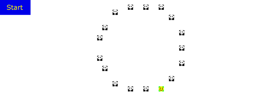
Start this macro by deleting the old button, the one that starts the simulation, I will replace it with a new button that reads “Start” to signify the new begging. Place and size it using the parameters I explained in the above paragraph, I placed mine in cell A1. Using the OnAction command set it to run macro “rotate” which sets up the whole simulation all over again.
Sub endsim()
Application.ScreenUpdating = False
ActiveSheet.Pictures("rs").Delete
viscols = ActiveWindow.VisibleRange.Columns.Count
visrows = ActiveWindow.VisibleRange.Rows.Count
width1 = Int(viscols / 8)
height1 = Int(visrows / 4)
Picture = "C:\Users\Rik7000\Desktop\Ex-Cell games\start.png"
With Cells(1, 1)
Set mypic = ActiveSheet.Pictures.Insert(Picture)
mypic.Top = .Top
mypic.Left = .Left
mypic.Width = .Width
mypic.Height = .Height
mypic.Name = "rs"
mypic.OnAction = "Module1.rotate"
End With
ActiveSheet.Pictures("rs").Height = Sheet1.Range(Cells(1, 1), Cells(height1, 1)).Height
ActiveSheet.Pictures("rs").Width = Sheet1.Range(Cells(1, 1), Cells(1, width1)).Width
Application.ScreenUpdating = True
End Sub
As promised, here is the final macro, “reset.” This runs every time a new simulation is requested. It simply deletes all pictures on the sheet and resets the cells’ value and color to “” and white.
Sub reset()
Cells.Value = ""
Cells.Interior.ColorIndex = 2
ActiveSheet.Pictures.Delete
Range("A1").Select
End Sub
Once all of that is in place and working together in harmony you can run a simulation of any size that Excel will allow. This ends the simulation portion.
For the next section we will be using an equation to calculate the winning seat and spit out the answer, this of course allows for the calculation of much, much larger values of n.
Part 2: General Solution with Equation
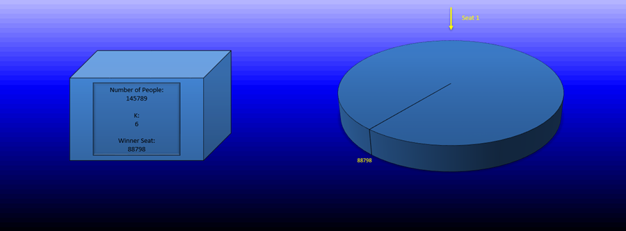
This sheet is comprised of a cube displaying three numbers, number of people (n), the K value, and the winning seat. Next to the cube is a pie chart that will show the relative position of the winning seat to seat 1, so you can see how far around the circle the winner is. That is achieved by rotating the pie slice which will be explained below.
First let’s look at the general equation used to solve the Josephus problem with an arbitrary K value. This equation is dynamic, meaning it will loop through and find the value of D that satisfies the requirement that the ceiling value of (k/k-1)*D is less than or equal to (k-1)n.
�=1
While �≤(�−1)�
�=⌈�(�−1)∗�⌉
The winning seat is then given by:
������=��+1–�
And now for the VBA. Collect two inputs from the user using the application.inputbox method. We will need an n and a K value. After obtaining those, simply plug the values into the equation.
Sub findwinner()
Dim winner As Double
Dim n As Double
Application.ScreenUpdating = False
n = Application.InputBox("Please enter the number of people")
k = Application.InputBox("Please enter the K value.")
D = 1
Do While D <= (k - 1) * n
D = WorksheetFunction.RoundUp((k / (k - 1)) * D, 0)
Loop
winner = k * n + 1 - D
Once a winner has been calculated, store that value in cell Y3 to be used by the sheet later. Also store n in a cell, mine is Y1
Range("Y1").Value = n
Range("Y3").Value = winner
Next calculate the percent that the pie chart slice needs to be rotated. I also move the slice back by one so that seat 1 is always in the same position on the pie chart. Simply divide the winning seat number by the total number of people to get the percentage around the circle, then subtract off another slice. One slice is simply 1/n. After that, rotate the first slice of the pie chart by the correct amount which is of course the percentage we desire times 360 (because there are 360 degrees around the circle).
perc = ((winner / n) - (1 / n))
ActiveSheet.ChartObjects("Chart 3").Activate
ActiveChart.ChartGroups(1).FirstSliceAngle = perc * 360
Range("A1").Select
The next step is to simply display the data on the cube. Inside the cube I placed another shape, with that shape the text is centered and formatted how I like so all the macro has to do is change the values. You can see it doing that below, note that using “_ “ denotes a line break. Also remember that inserting a variable into a string of text is easy using “ & “ (for example: “This is string number “ & [variable] & “, pretty cool, uh?”).
Sheets(2).Shapes("textbox 14").TextFrame.Characters.Text = "Number of People:" _
& Chr(13) & n _
& Chr(13) _
& Chr(13) & "K:" _
& Chr(13) _
& q _
& Chr(13) _
& Chr(13) _
& "Winner Seat:" & Chr(13) _
& winner
Application.ScreenUpdating = True
End Sub
I have my macro run whenever the user clicks on the cube. That concludes the second part, the final part calculates the winning seat for any given K value for n from 1 to an arbitrary number and plots the winning seats. This allows you to see the patterns of winners produced by different K values.
Part 3: Plotting the Winning Seats
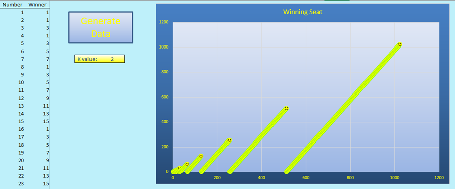
After making the background a light blue, insert a graph. The data for the graph should be column B from B2 to any other B value, this will become a variable anyway. Cell E8 will display the K value so format that as you wish and insert a button that triggers the macro “create_data.” Set nstop and k as variable type double (nstop is for the largest n value the user wants and k is for K). First clear the old data held in columns A and B, next insert the column headers “Number” and “Winner” in A1 and B1 respectively. This time n always starts as 1 so obtain from the user the largest value of n desired and the program will calculate the winners for each n value up to that number. Grab the K value as well before moving on.
Sub create_data()
Dim nstop As Double
Dim k As Double
Columns("A:B").ClearContents
Range("A1").Value = "Number"
Range("B1").Value = "Winner"
n = 1
nstop = Application.InputBox("Please enter the largest n")
k = Application.InputBox("Enter k")
The program should now loop until n = nstop + 1. Add 1 to nstop to ensure that the program includes the number entered by the user, if they enter 100 the program will not enter the loop once n = 100 and only 99 numbers will be presented. By adding 1 the program cuts out when n = 101 ensuring that the 100th loop is completed. You will see that loop below and once again I will be using the equation to determine the winning seat. Simply plug in the K value and perform the calculation for n = 1 to the user entered breaking point. Easy!
Do Until n = nstop + 1
D = 1
Do While D <= (k - 1) * n
D = WorksheetFunction.RoundUp((k / (k - 1)) * D, 0)
Loop
winner = k * n + 1 - D
Make sure to print out each n value and corresponding winning seat in columns A and B respectively, this way we can see the winners for each n value and we can have the graph pick up the data and display the pattern for us. Also, display the chosen K value so that we know what we are looking at.
Sheets("Winning Seats").Cells(n + 1, 1).Value = n
Sheets("Winning Seats").Cells(n + 1, 2).Value = winner
n = n + 1
Loop
Sheets("Winning Seats").Range("E8").Value = k
Finally, it’s time to adjust the graph. I want the graph to display the number of elements calculated after each run. So if the user wants 1 to 10 then the graph should display only 10 rows of data. If the user selects 1 to 12,349 then I want my graph to display 12,349 rows’ worth of data. In order to the that I need to obtain the last row with data in it and adjust the data displayed by my graph so that it captures everything from B2 to the final row, no more, no less. The familiar way is to use a row count function and xlUp.
lastr = Cells(Rows.Count, "A").End(xlUp).Row
Then manually change the graph’s data source using the new variable as the last row holding the data.
ActiveSheet.ChartObjects("Chart 2").Chart.SetSourceData Source:=Range("B2:B" & lastr)
End Sub
Now you can play around with the different K values and observe the difference on the graph.
That is just about it for the Josephus Problem which, I think, is a pretty interesting logic problem. I hope you enjoyed learning how to create this and that you will also have fun running the simulation and looking at the patterns in the graphs as well.
Download the Excel file and other images here: